Getting Started
Table of contents:
Installation
Sgkit itself contains only Python code but many of the required dependencies use compiled code or have system package dependencies. For this reason, conda is the preferred installation method. There is no sgkit conda package yet though so the recommended setup instructions are:
$ conda install -c conda-forge --file requirements.txt
$ pip install --pre sgkit
Overview
Sgkit is a general purpose toolkit for quantitative and population genetics. The primary goal of sgkit is to take advantage of powerful tools in the PyData ecosystem to facilitate interactive analysis of large-scale datasets. The main libraries we use are:
Xarray: N-D labeling for arrays and datasets
Dask: Parallel computing on chunked arrays
Zarr: Storage for chunked arrays
Numpy: N-D in-memory array manipulation
Pandas: Tabular data frame manipulation
CuPy: Numpy-like array interface for CUDA GPUs
Data structures
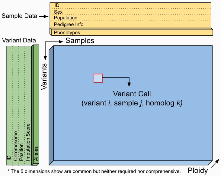
Sgkit uses Xarray Dataset objects to model genetic data.
Users are free to manipulate quantities within these objects as they see fit and a set of conventions for variable names,
dimensions and underlying data types is provided to aid in workflow standardization. The example below illustrates a
Dataset format that would result from an assay expressible as VCF,
PLINK or BGEN.
This is a guideline however, and a Dataset seen in practice might include many more or fewer variables and dimensions.
The worked examples below show how to access and visualize data like this using Xarray. They also demonstrate several of the sgkit conventions in place for representing common genetic quantities.
In [1]: import sgkit as sg

In [2]: ds = sg.simulate_genotype_call_dataset(n_variant=1000, n_sample=250, n_contig=23, missing_pct=.1)

In [3]: ds
Out[3]:
<xarray.Dataset>
Dimensions:             (alleles: 2, ploidy: 2, samples: 250, variants: 1000)
Dimensions without coordinates: alleles, ploidy, samples, variants
Data variables:
    variant_contig      (variants) int64 0 0 0 0 0 0 0 ... 22 22 22 22 22 22 22
    variant_position    (variants) int64 0 1 2 3 4 5 6 ... 36 37 38 39 40 41 42
    variant_allele      (variants, alleles) |S1 b'G' b'A' b'T' ... b'A' b'T'
    sample_id           (samples) <U4 'S0' 'S1' 'S2' ... 'S247' 'S248' 'S249'
    call_genotype       (variants, samples, ploidy) int8 0 0 1 0 1 ... 0 0 0 0 1
    call_genotype_mask  (variants, samples, ploidy) bool False False ... False
Attributes:
    contigs:  [0, 1, 2, 3, 4, 5, 6, 7, 8, 9, 10, 11, 12, 13, 14, 15, 16, 17, ...
The presence of a single-nucleotide variant (SNV) is indicated above by the call_genotype variable, which contains
an integer value corresponding to the index of the associated allele present (i.e. index into the variant_allele variable)
for a sample at a given genome coordinate and chromosome. Every sgkit variable has a set of fixed semantics like this. For more
information on this specific variable and any others, see Genetic variables.
Data subsets can be accessed as shown here, using the features described in Indexing and Selecting Xarray Data:
In [4]: import sgkit as sg

In [5]: ds = sg.simulate_genotype_call_dataset(n_variant=100, n_sample=50, n_contig=23, missing_pct=.1)

# Subset the entire dataset to the first 10 variants/samples
In [6]: ds.isel(variants=slice(10), samples=slice(10))
Out[6]:
<xarray.Dataset>
Dimensions:             (alleles: 2, ploidy: 2, samples: 10, variants: 10)
Dimensions without coordinates: alleles, ploidy, samples, variants
Data variables:
    variant_contig      (variants) int64 0 0 0 0 0 1 1 1 1 1
    variant_position    (variants) int64 0 1 2 3 4 0 1 2 3 4
    variant_allele      (variants, alleles) |S1 b'T' b'C' b'C' ... b'T' b'A'
    sample_id           (samples) <U3 'S0' 'S1' 'S2' 'S3' ... 'S7' 'S8' 'S9'
    call_genotype       (variants, samples, ploidy) int8 0 0 1 0 1 ... 0 1 1 1 1
    call_genotype_mask  (variants, samples, ploidy) bool False False ... False
Attributes:
    contigs:  [0, 1, 2, 3, 4, 5, 6, 7, 8, 9, 10, 11, 12, 13, 14, 15, 16, 17, ...

# Subset to a specific set of variables
In [7]: ds[['variant_allele', 'call_genotype']]
Out[7]:
<xarray.Dataset>
Dimensions:         (alleles: 2, ploidy: 2, samples: 50, variants: 100)
Dimensions without coordinates: alleles, ploidy, samples, variants
Data variables:
    variant_allele  (variants, alleles) |S1 b'T' b'C' b'C' ... b'T' b'T' b'A'
    call_genotype   (variants, samples, ploidy) int8 0 0 1 0 1 0 ... 0 1 0 1 0 0
Attributes:
    contigs:  [0, 1, 2, 3, 4, 5, 6, 7, 8, 9, 10, 11, 12, 13, 14, 15, 16, 17, ...

# Extract a single variable
In [8]: ds.call_genotype[:3, :3]
Out[8]:
<xarray.DataArray 'call_genotype' (variants: 3, samples: 3, ploidy: 2)>
array([[[ 0,  0],
        [ 1,  0],
        [ 1,  0]],

       [[ 1,  1],
        [ 1,  0],
        [ 1, -1]],

       [[ 0,  1],
        [ 1,  1],
        [ 1,  1]]], dtype=int8)
Dimensions without coordinates: variants, samples, ploidy
Attributes:
    mixed_ploidy:  False

# Access the array underlying a single variable (this would return dask.array.Array if chunked)
In [9]: ds.call_genotype.data[:3, :3]
Out[9]:
array([[[ 0,  0],
        [ 1,  0],
        [ 1,  0]],

       [[ 1,  1],
        [ 1,  0],
        [ 1, -1]],

       [[ 0,  1],
        [ 1,  1],
        [ 1,  1]]], dtype=int8)

# Access the alleles corresponding to the calls for the first variant and sample
In [10]: allele_indexes = ds.call_genotype[0, 0]

In [11]: allele_indexes
Out[11]:
<xarray.DataArray 'call_genotype' (ploidy: 2)>
array([0, 0], dtype=int8)
Dimensions without coordinates: ploidy
Attributes:
    mixed_ploidy:  False

In [12]: ds.variant_allele[0, allele_indexes]
Out[12]:
<xarray.DataArray 'variant_allele' (ploidy: 2)>
array([b'T', b'T'], dtype='|S1')
Dimensions without coordinates: ploidy

# Get a single item from an array as a Python scalar
In [13]: ds.sample_id.item(0)
Out[13]: 'S0'
Larger subsets of data can be visualized and/or summarized through various sgkit utilities as well as the Pandas/Xarray integration:
In [14]: import sgkit as sg

In [15]: ds = sg.simulate_genotype_call_dataset(n_variant=1000, n_sample=250, missing_pct=.1)

# Show genotype calls with domain-specific display logic
In [16]: sg.display_genotypes(ds, max_variants=8, max_samples=8)
Out[16]:
samples    S0   S1   S2 S245  ... S248 S249   S3   S4
variants                      ...
0         0/0  1/0  1/0  1/0  ...  1/1  1/0  0/1  ./0
1         0/0  0/1  1/1  0/1  ...  0/.  0/0  1/1  ./0
2         1/1  0/1  1/0  1/.  ...  0/1  ./1  0/1  1/0
3         1/0  1/0  1/0  0/0  ...  0/1  1/.  1/0  1/1
...       ...  ...  ...  ...  ...  ...  ...  ...  ...
996       0/.  1/1  1/1  1/1  ...  1/0  ./0  0/0  0/1
997       0/0  ./0  1/0  1/0  ...  1/1  ./1  1/1  ./1
998       0/1  0/1  1/1  0/0  ...  0/1  ./1  1/0  1/.
999       1/0  0/1  1/0  0/.  ...  0/0  0/1  1/1  0/1

[1000 rows x 250 columns]

# A naive version of the above is also possible using only Xarray/Pandas and
# illustrates the flexibility that comes from being able to transition into
# and out of array/dataframe representations easily
In [17]: (ds.call_genotype[:5, :5].to_series()
   ....:     .unstack().where(lambda df: df >= 0, None).fillna('.')
   ....:     .astype(str).apply('/'.join, axis=1).unstack())
   ....:
Out[17]:
samples     0    1    2    3    4
variants
0         0/0  1/0  1/0  0/1  ./0
1         0/0  0/1  1/1  1/1  ./0
2         1/1  0/1  1/0  0/1  1/0
3         1/0  1/0  1/0  1/0  1/1
4         ./1  ./1  1/1  0/0  0/1

# Show call rate distribution for each variant using Pandas
In [18]: df = ~ds.call_genotype_mask.to_dataframe()

In [19]: df.head(5)
Out[19]:
                         call_genotype_mask
variants samples ploidy
0        0       0                     True
                 1                     True
         1       0                     True
                 1                     True
         2       0                     True

In [20]: call_rates = df.groupby('variants').mean()

In [21]: call_rates
Out[21]:
          call_genotype_mask
variants
0                      0.898
1                      0.910
2                      0.926
3                      0.894
4                      0.892
...                      ...
995                    0.892
996                    0.906
997                    0.900
998                    0.900
999                    0.910

[1000 rows x 1 columns]

In [22]: call_rates.plot(kind='hist', bins=24, title='Call Rate Distribution', figsize=(6, 3))
Out[22]: <AxesSubplot:title={'center':'Call Rate Distribution'}, ylabel='Frequency'>
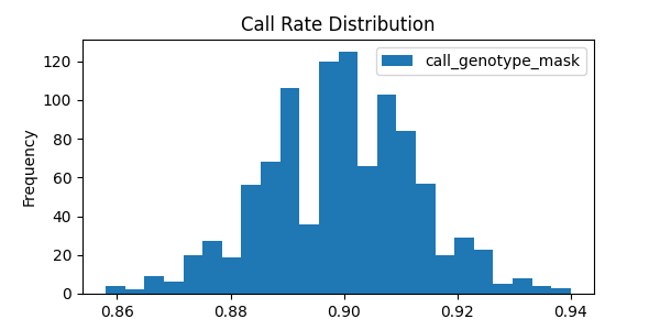
This last example alludes to representations of missing data that are explained further in Missing data.
Genetic methods
Genetic methods in sgkit are nearly always applied to individual Dataset objects. For a full list of
available methods, see Methods.
In this example, the variant_stats method is applied to a dataset to compute a number of statistics
across samples for each individual variant:
In [23]: import sgkit as sg

In [24]: ds = sg.simulate_genotype_call_dataset(n_variant=100, n_sample=50, missing_pct=.1)

In [25]: sg.variant_stats(ds, merge=False)
Out[25]:
<xarray.Dataset>
Dimensions:                   (alleles: 2, variants: 100)
Dimensions without coordinates: alleles, variants
Data variables:
    variant_n_called          (variants) int64 40 42 43 40 41 ... 42 38 43 43 40
    variant_call_rate         (variants) float64 0.8 0.84 0.86 ... 0.86 0.86 0.8
    variant_n_het             (variants) int64 22 30 18 26 29 ... 23 22 26 21 19
    variant_n_hom_ref         (variants) int64 11 3 13 3 6 8 ... 6 10 9 12 8 13
    variant_n_hom_alt         (variants) int64 7 9 12 11 6 17 ... 15 9 7 5 14 8
    variant_n_non_ref         (variants) int64 29 39 30 37 35 ... 32 29 31 35 27
    variant_allele_count      (variants, alleles) uint64 dask.array<chunksize=(100, 2), meta=np.ndarray>
    variant_allele_total      (variants) int64 90 92 93 88 91 ... 92 88 92 92 90
    variant_allele_frequency  (variants, alleles) float64 dask.array<chunksize=(100, 2), meta=np.ndarray>
There are two ways that the results of every function are handled – either they are merged with the provided dataset or they are returned in a separate dataset. See Dataset merge behavior below for more details.
Dataset merge behavior
Generally, method functions in sgkit compute some new variables based on the input dataset, then return a new output dataset that consists of the input dataset plus the new computed variables. The input dataset is unchanged.
This behavior can be controlled using the merge parameter. If set to True
(the default), then the function will merge the input dataset and the computed
output variables into a single dataset. Output variables will overwrite any
input variables with the same name, and a warning will be issued in this case.
If False, the function will return only the computed output variables.
Examples:
In [26]: import sgkit as sg

In [27]: ds = sg.simulate_genotype_call_dataset(n_variant=100, n_sample=50, missing_pct=.1)

In [28]: ds = ds[['variant_allele', 'call_genotype']]

In [29]: ds
Out[29]:
<xarray.Dataset>
Dimensions:         (alleles: 2, ploidy: 2, samples: 50, variants: 100)
Dimensions without coordinates: alleles, ploidy, samples, variants
Data variables:
    variant_allele  (variants, alleles) |S1 b'T' b'C' b'C' ... b'T' b'T' b'A'
    call_genotype   (variants, samples, ploidy) int8 0 0 1 0 1 0 ... 0 1 0 1 0 0
Attributes:
    contigs:  [0]

# By default, new variables are merged into a copy of the provided dataset
In [30]: ds = sg.count_variant_alleles(ds)

In [31]: ds
Out[31]:
<xarray.Dataset>
Dimensions:               (alleles: 2, ploidy: 2, samples: 50, variants: 100)
Dimensions without coordinates: alleles, ploidy, samples, variants
Data variables:
    variant_allele_count  (variants, alleles) uint64 dask.array<chunksize=(100, 2), meta=np.ndarray>
    call_allele_count     (variants, samples, alleles) uint8 dask.array<chunksize=(100, 50, 2), meta=np.ndarray>
    variant_allele        (variants, alleles) |S1 b'T' b'C' b'C' ... b'T' b'A'
    call_genotype         (variants, samples, ploidy) int8 0 0 1 0 1 ... 0 1 0 0
Attributes:
    contigs:  [0]

# If an existing variable would be re-defined, a warning is thrown
In [32]: import warnings

In [33]: ds = sg.count_variant_alleles(ds)

In [34]: with warnings.catch_warnings(record=True) as w:
   ....:     ds = sg.count_variant_alleles(ds)
   ....:     print(f"{w[0].category.__name__}: {w[0].message}")
   ....:
MergeWarning: The following variables in the input dataset will be replaced in the output: variant_allele_count

# New variables can also be returned in their own dataset
In [35]: sg.count_variant_alleles(ds, merge=False)
Out[35]:
<xarray.Dataset>
Dimensions:               (alleles: 2, variants: 100)
Dimensions without coordinates: alleles, variants
Data variables:
    variant_allele_count  (variants, alleles) uint64 dask.array<chunksize=(100, 2), meta=np.ndarray>

# This can be useful for merging multiple datasets manually
In [36]: ds.merge(sg.count_variant_alleles(ds, merge=False))
Out[36]:
<xarray.Dataset>
Dimensions:               (alleles: 2, ploidy: 2, samples: 50, variants: 100)
Dimensions without coordinates: alleles, ploidy, samples, variants
Data variables:
    variant_allele_count  (variants, alleles) uint64 dask.array<chunksize=(100, 2), meta=np.ndarray>
    call_allele_count     (variants, samples, alleles) uint8 dask.array<chunksize=(100, 50, 2), meta=np.ndarray>
    variant_allele        (variants, alleles) |S1 b'T' b'C' b'C' ... b'T' b'A'
    call_genotype         (variants, samples, ploidy) int8 0 0 1 0 1 ... 0 1 0 0
Attributes:
    contigs:  [0]
Missing data
Missing data in sgkit is represented using a sentinel value within data arrays
(-1 in integer arrays and NaN in float arrays) as well as a companion boolean mask array
(True where data is missing). These sentinel values are handled transparently in
most sgkit functions and where this isn’t possible, limitations related to it are documented
along with potential workarounds.
This example demonstrates one such function where missing calls are ignored:
In [37]: import sgkit as sg

In [38]: ds = sg.simulate_genotype_call_dataset(n_variant=1, n_sample=4, n_ploidy=2, missing_pct=.3, seed=4)

In [39]: ds.call_genotype
Out[39]:
<xarray.DataArray 'call_genotype' (variants: 1, samples: 4, ploidy: 2)>
array([[[ 0,  0],
        [ 1,  1],
        [-1,  0],
        [-1, -1]]], dtype=int8)
Dimensions without coordinates: variants, samples, ploidy
Attributes:
    mixed_ploidy:  False

# Here, you can see that the missing calls above are not included in the allele counts
In [40]: sg.count_variant_alleles(ds).variant_allele_count
Out[40]:
<xarray.DataArray 'variant_allele_count' (variants: 1, alleles: 2)>
dask.array<sum-aggregate, shape=(1, 2), dtype=uint64, chunksize=(1, 2), chunktype=numpy.ndarray>
Dimensions without coordinates: variants, alleles
A primary design goal in sgkit is to facilitate ad hoc analysis. There are many useful functions in the library but they are not enough on their own to accomplish many analyses. To that end, it is often helpful to be able to handle missing data in your own functions or exploratory summaries. Both the sentinel values and the boolean mask array help make this possible, where the sentinel values are typically more useful when implementing compiled operations and the boolean mask array is easier to use in a higher level API like Xarray or Numpy. Only advanced users would likely ever need to worry about compiling their own functions (see Custom Computations for more details). Using Xarray functions and the boolean mask is generally enough to accomplish most tasks, and this mask is often more efficient to operate on due to its high on-disk compression ratio. This example shows how it can be used in the context of doing something simple like counting heterozygous calls:
In [41]: import sgkit as sg

In [42]: import xarray as xr

In [43]: ds = sg.simulate_genotype_call_dataset(n_variant=1, n_sample=4, n_ploidy=2, missing_pct=.2, seed=2)

# This array contains the allele indexes called for a sample
In [44]: ds.call_genotype
Out[44]:
<xarray.DataArray 'call_genotype' (variants: 1, samples: 4, ploidy: 2)>
array([[[-1,  0],
        [ 1,  1],
        [ 1,  0],
        [ 1,  1]]], dtype=int8)
Dimensions without coordinates: variants, samples, ploidy
Attributes:
    mixed_ploidy:  False

# This array represents only locations where the above calls are missing
In [45]: ds.call_genotype_mask
Out[45]:
<xarray.DataArray 'call_genotype_mask' (variants: 1, samples: 4, ploidy: 2)>
array([[[ True, False],
        [False, False],
        [False, False],
        [False, False]]])
Dimensions without coordinates: variants, samples, ploidy

# Determine which calls are heterozygous
In [46]: is_heterozygous = (ds.call_genotype[..., 0] != ds.call_genotype[..., 1])

In [47]: is_heterozygous
Out[47]:
<xarray.DataArray 'call_genotype' (variants: 1, samples: 4)>
array([[ True, False,  True, False]])
Dimensions without coordinates: variants, samples

# Count the number of heterozygous samples for the lone variant
In [48]: is_heterozygous.sum().item(0)
Out[48]: 2

# This is almost correct except that the calls for the first sample aren't
# really heterozygous, one of them is just missing.  Conditional logic like
# this can be used to isolate those values and replace them in the result:
In [49]: xr.where(ds.call_genotype_mask.any(dim='ploidy'), False, is_heterozygous).sum().item(0)
Out[49]: 1

# Now the result is correct -- only the third sample is heterozygous so the count should be 1.
# This how many sgkit functions handle missing data internally:
In [50]: sg.variant_stats(ds).variant_n_het.item(0)
Out[50]: 1
Chaining operations
Method chaining is a common practice with Python data tools that improves code readability and reduces the probability of introducing accidental namespace collisions. Sgkit functions are compatible with this idiom by default and this example shows to use it in conjunction with Xarray and Pandas operations in a single pipeline:
In [51]: import sgkit as sg

In [52]: ds = sg.simulate_genotype_call_dataset(n_variant=100, n_sample=50, missing_pct=.1)

# Use `pipe` to apply a single sgkit function to a dataset
In [53]: ds_qc = ds.pipe(sg.variant_stats).drop_dims('samples')

In [54]: ds_qc
Out[54]:
<xarray.Dataset>
Dimensions:                   (alleles: 2, variants: 100)
Dimensions without coordinates: alleles, variants
Data variables:
    variant_n_called          (variants) int64 40 42 43 40 41 ... 42 38 43 43 40
    variant_call_rate         (variants) float64 0.8 0.84 0.86 ... 0.86 0.86 0.8
    variant_n_het             (variants) int64 22 30 18 26 29 ... 23 22 26 21 19
    variant_n_hom_ref         (variants) int64 11 3 13 3 6 8 ... 6 10 9 12 8 13
    variant_n_hom_alt         (variants) int64 7 9 12 11 6 17 ... 15 9 7 5 14 8
    variant_n_non_ref         (variants) int64 29 39 30 37 35 ... 32 29 31 35 27
    variant_allele_count      (variants, alleles) uint64 dask.array<chunksize=(100, 2), meta=np.ndarray>
    variant_allele_total      (variants) int64 90 92 93 88 91 ... 92 88 92 92 90
    variant_allele_frequency  (variants, alleles) float64 dask.array<chunksize=(100, 2), meta=np.ndarray>
    variant_contig            (variants) int64 0 0 0 0 0 0 0 0 ... 0 0 0 0 0 0 0
    variant_position          (variants) int64 0 1 2 3 4 5 ... 94 95 96 97 98 99
    variant_allele            (variants, alleles) |S1 b'T' b'C' ... b'T' b'A'
Attributes:
    contigs:  [0]

# Show statistics for one of the arrays to be used as a filter
In [55]: ds_qc.variant_call_rate.to_series().describe()
Out[55]:
count    100.000000
mean       0.804800
std        0.063125
min        0.560000
25%        0.780000
50%        0.800000
75%        0.840000
max        0.960000
Name: variant_call_rate, dtype: float64

# Build a pipeline that filters on call rate and computes Fst between two cohorts
In [56]: (
   ....:     ds
   ....:     .pipe(sg.variant_stats)
   ....:     .pipe(lambda ds: ds.sel(variants=ds.variant_call_rate > .8))
   ....:     .assign(sample_cohort=np.repeat([0, 1], ds.dims['samples'] // 2))
   ....:     .pipe(sg.Fst)
   ....:     .stat_Fst.values
   ....: )
   ....:
Out[56]:
array([[[        nan, -0.01262437],
        [-0.01262437,         nan]],

       [[        nan,  0.11508453],
        [ 0.11508453,         nan]],

       [[        nan, -0.01641002],
        [-0.01641002,         nan]],

       [[        nan, -0.01070192],
        [-0.01070192,         nan]],

       [[        nan, -0.01343231],
        [-0.01343231,         nan]],

       [[        nan, -0.02170543],
        [-0.02170543,         nan]],

       [[        nan, -0.015625  ],
        [-0.015625  ,         nan]],

       [[        nan,  0.04508451],
        [ 0.04508451,         nan]],

       [[        nan, -0.00788022],
        [-0.00788022,         nan]],

       [[        nan, -0.02200358],
        [-0.02200358,         nan]],

       [[        nan,  0.01818182],
        [ 0.01818182,         nan]],

       [[        nan, -0.02074074],
        [-0.02074074,         nan]],

       [[        nan,  0.03048181],
        [ 0.03048181,         nan]],

       [[        nan,  0.01223471],
        [ 0.01223471,         nan]],

       [[        nan,  0.00679281],
        [ 0.00679281,         nan]],

       [[        nan, -0.00726744],
        [-0.00726744,         nan]],

       [[        nan, -0.01991852],
        [-0.01991852,         nan]],

       [[        nan, -0.02219873],
        [-0.02219873,         nan]],

       [[        nan, -0.01061008],
        [-0.01061008,         nan]],

       [[        nan, -0.0207084 ],
        [-0.0207084 ,         nan]],

       [[        nan,  0.0067726 ],
        [ 0.0067726 ,         nan]],

       [[        nan,  0.04660046],
        [ 0.04660046,         nan]],

       [[        nan, -0.00082034],
        [-0.00082034,         nan]],

       [[        nan, -0.01352657],
        [-0.01352657,         nan]],

       [[        nan,  0.00201873],
        [ 0.00201873,         nan]],

       [[        nan,  0.0110247 ],
        [ 0.0110247 ,         nan]],

       [[        nan, -0.011512  ],
        [-0.011512  ,         nan]],

       [[        nan, -0.01310332],
        [-0.01310332,         nan]],

       [[        nan, -0.02020202],
        [-0.02020202,         nan]],

       [[        nan,  0.00212987],
        [ 0.00212987,         nan]],

       [[        nan, -0.02232511],
        [-0.02232511,         nan]],

       [[        nan,  0.04404655],
        [ 0.04404655,         nan]],

       [[        nan, -0.01800334],
        [-0.01800334,         nan]],

       [[        nan,  0.00213303],
        [ 0.00213303,         nan]],

       [[        nan, -0.020855  ],
        [-0.020855  ,         nan]],

       [[        nan, -0.01168929],
        [-0.01168929,         nan]],

       [[        nan,  0.05730659],
        [ 0.05730659,         nan]],

       [[        nan,  0.07480478],
        [ 0.07480478,         nan]],

       [[        nan, -0.01535189],
        [-0.01535189,         nan]],

       [[        nan,  0.01204221],
        [ 0.01204221,         nan]],

       [[        nan, -0.01860705],
        [-0.01860705,         nan]],

       [[        nan,  0.02312629],
        [ 0.02312629,         nan]],

       [[        nan, -0.02123361],
        [-0.02123361,         nan]]])
This is possible because sgkit functions nearly always take a Dataset as the first argument, create new
variables, and then merge these new variables into a copy of the provided dataset in the returned value.
See Dataset merge behavior for more details.
Chunked arrays
Chunked arrays are required when working on large datasets. Libraries for managing chunked arrays such as Dask Array and Zarr make it possible to implement blockwise algorithms that operate on subsets of arrays (in parallel) without ever requiring them to fit entirely in memory.
By design, they behave almost identically to in-memory (typically Numpy) arrays within Xarray and can be interchanged freely when provided
to sgkit functions. The most notable difference in behavior though is that operations on chunked arrays are evaluated lazily.
This means that if an Xarray Dataset contains only chunked arrays, no actual computations will be performed
until one of the following occurs:
Dataset.compute is called
DataArray.compute is called
The
DataArray.valuesattribute is referencedIndividual dask arrays are retrieved through the
DataArray.dataattribute and forced to evaluate via Client.compute, dask.array.Array.compute or by coercing them to another array type (e.g. using np.asarray)
This example shows a few of these features:
In [57]: import sgkit as sg

In [58]: ds = sg.simulate_genotype_call_dataset(n_variant=100, n_sample=50, missing_pct=.1)

# Chunk our original in-memory dataset using a blocksize of 50 in all dimensions.
In [59]: ds = ds.chunk(chunks=50)

In [60]: ds
Out[60]:
<xarray.Dataset>
Dimensions:             (alleles: 2, ploidy: 2, samples: 50, variants: 100)
Dimensions without coordinates: alleles, ploidy, samples, variants
Data variables:
    variant_contig      (variants) int64 dask.array<chunksize=(50,), meta=np.ndarray>
    variant_position    (variants) int64 dask.array<chunksize=(50,), meta=np.ndarray>
    variant_allele      (variants, alleles) |S1 dask.array<chunksize=(50, 2), meta=np.ndarray>
    sample_id           (samples) <U3 dask.array<chunksize=(50,), meta=np.ndarray>
    call_genotype       (variants, samples, ploidy) int8 dask.array<chunksize=(50, 50, 2), meta=np.ndarray>
    call_genotype_mask  (variants, samples, ploidy) bool dask.array<chunksize=(50, 50, 2), meta=np.ndarray>
Attributes:
    contigs:  [0]

# Show the chunked array representing base pair position
In [61]: ds.variant_position
Out[61]:
<xarray.DataArray 'variant_position' (variants: 100)>
dask.array<xarray-variant_position, shape=(100,), dtype=int64, chunksize=(50,), chunktype=numpy.ndarray>
Dimensions without coordinates: variants

# Call compute via the dask.array API
In [62]: ds.variant_position.data.compute()[:5]
Out[62]: array([0, 1, 2, 3, 4])

# Coerce to numpy via Xarray
In [63]: ds.variant_position.values[:5]
Out[63]: array([0, 1, 2, 3, 4])

# Compute without unboxing from xarray.DataArray
In [64]: ds.variant_position.compute()[:5]
Out[64]:
<xarray.DataArray 'variant_position' (variants: 5)>
array([0, 1, 2, 3, 4])
Dimensions without coordinates: variants
Unlike this simplified example, real datasets often contain a mixture of chunked and unchunked arrays. Sgkit
will often load smaller arrays directly into memory while leaving large arrays chunked as a trade-off between
convenience and resource usage. This can always be modified by users though and sgkit functions that operate
on a Dataset should work regardless of the underlying array backend.
See Parallel computing with Dask in Xarray for more examples and information, as well as the Dask tutorials on delayed array execution and lazy execution in Dask graphs.
Monitoring operations
The simplest way to monitor operations when running sgkit on a single host is to use Dask local diagnostics.
As an example, this code shows how to track the progress of a single sgkit function:
In [65]: import sgkit as sg

In [66]: from dask.diagnostics import ProgressBar

In [67]: ds = sg.simulate_genotype_call_dataset(n_variant=100, n_sample=50, missing_pct=.1)

In [68]: with ProgressBar():
   ....:     ac = sg.count_variant_alleles(ds).variant_allele_count.compute()
   ....:

[                                        ] | 0% Completed |  0.0s
[########################################] | 100% Completed |  0.1s

In [69]: ac[:5]
Out[69]:
<xarray.DataArray 'variant_allele_count' (variants: 5, alleles: 2)>
array([[50, 40],
       [40, 52],
       [48, 45],
       [37, 51],
       [45, 46]], dtype=uint64)
Dimensions without coordinates: variants, alleles
Monitoring resource utilization with ResourceProfiler and profiling task streams with Profiler are other commonly used local diagnostics.
For similar monitoring in a distributed cluster, see Dask distributed diagnostics.
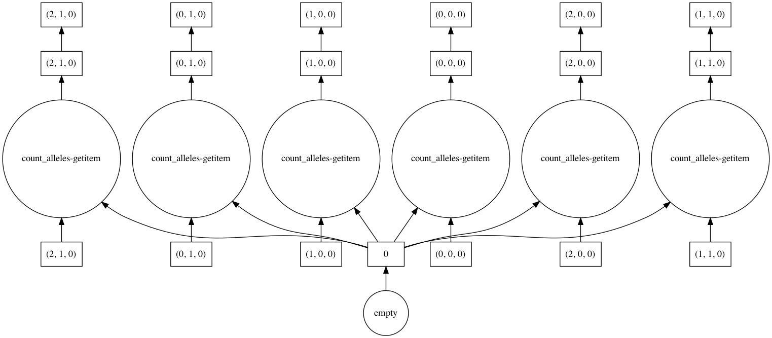
Visualizing computations
Dask allows you to visualize the task graph of a computation before running it, which can be handy when trying to understand where the bottlenecks are.
In most cases the number of tasks is too large to visualize, so it’s useful to restrict the graph just a few chunks, as shown in this example.
In [70]: import sgkit as sg

In [71]: ds = sg.simulate_genotype_call_dataset(n_variant=100, n_sample=50, missing_pct=.1)

# Rechunk to illustrate multiple tasks
In [72]: ds = ds.chunk({"variants": 25, "samples": 25})

In [73]: counts = sg.count_call_alleles(ds).call_allele_count.data

# Restrict to first 3 chunks in variants dimension
In [74]: counts = counts[:3*counts.chunksize[0],...]

In [75]: counts.visualize(optimize_graph=True)
Out[75]: <IPython.core.display.Image object>
By passing keyword arguments to visualize we can see the order tasks will run in:
# Graph where colors indicate task ordering
In [76]: counts.visualize(filename="order", optimize_graph=True, color="order", cmap="autumn", node_attr={"penwidth": "4"})
Out[76]: <IPython.core.display.Image object>
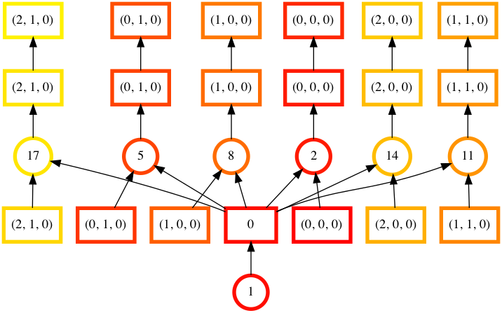
Task order number is shown in circular boxes, colored from red to yellow.
Custom naming conventions
TODO: Show to use a custom naming convention via Xarray renaming features.
Genetic variables
TODO: Link to and explain sgkit.variables in https://github.com/pystatgen/sgkit/pull/276.
Reading genetic data
TODO: Explain sgkit-{plink,vcf,bgen} once repos are consolidated and move this to a more prominent position in the docs.