GWAS Tutorial#
This notebook is an sgkit port of Hail’s GWAS Tutorial, which demonstrates how to run a genome-wide SNP association test. Readers are encouraged to read the Hail tutorial alongside this one for more background, and to see the motivation behind some of the steps.
Note that some of the results do not exactly match the output from Hail. Also, since sgkit is still a 0.x release, its API is still subject to non-backwards compatible changes.
import sgkit as sg
from sgkit.io.vcf import vcf_to_zarr
Before using sgkit, we import some standard Python libraries and set the Xarray display options to not show all the attributes in a dataset by default.
import numpy as np
import pandas as pd
import xarray as xr
xr.set_options(display_expand_attrs=False, display_expand_data_vars=True);
Download public 1000 Genomes data#
We use the same small (20MB) portion of the public 1000 Genomes data that Hail uses.
First, download the file locally:
from pathlib import Path
import requests

if not Path("1kg.vcf.bgz").exists():
    response = requests.get("https://storage.googleapis.com/sgkit-gwas-tutorial/1kg.vcf.bgz")
    with open("1kg.vcf.bgz", "wb") as f:
        f.write(response.content)
Importing data from VCF#
Next, convert it to Zarr, stored on the local filesystem in a directory called 1kg.zarr.
vcf_to_zarr("1kg.vcf.bgz", "1kg.zarr", max_alt_alleles=1,
          fields=["FORMAT/GT", "FORMAT/DP", "FORMAT/GQ", "FORMAT/AD"],
          field_defs={"FORMAT/AD": {"Number": "R"}})
[W::bcf_hdr_check_sanity] PL should be declared as Number=G
We passed a few arguments to the vcf_to_zarr conversion function, so it only converts the first alternate allele (max_alt_alleles=1), and to load extra VCF fields we are interested in (GT, DP, GQ, and AD). Also, AD needed defining as having a Number definition of R (one value for each allele, including the reference), since the dataset we are using defines it as . which means “unknown”.
Now the data has been written as Zarr, all downstream operations on will be much faster. Note that sgkit uses an Xarray dataset to represent the VCF data, where Hail uses MatrixTable.
ds = sg.load_dataset("1kg.zarr")
Getting to know our data#
To start with we’ll look at some summary data from the dataset.
The simplest thing is to look at the dimensions and data variables in the Xarray dataset.
ds
<xarray.Dataset>
Dimensions:               (variants: 10879, samples: 284, alleles: 2,
                           ploidy: 2, contigs: 84, filters: 1)
Dimensions without coordinates: variants, samples, alleles, ploidy, contigs,
                                filters
Data variables: (12/17)
    call_AD               (variants, samples, alleles) int32 dask.array<chunksize=(10000, 284, 2), meta=np.ndarray>
    call_DP               (variants, samples) int32 dask.array<chunksize=(10000, 284), meta=np.ndarray>
    call_GQ               (variants, samples) int32 dask.array<chunksize=(10000, 284), meta=np.ndarray>
    call_genotype         (variants, samples, ploidy) int8 dask.array<chunksize=(10000, 284, 2), meta=np.ndarray>
    call_genotype_mask    (variants, samples, ploidy) bool dask.array<chunksize=(10000, 284, 2), meta=np.ndarray>
    call_genotype_phased  (variants, samples) bool dask.array<chunksize=(10000, 284), meta=np.ndarray>
    ...                    ...
    variant_contig        (variants) int8 dask.array<chunksize=(10000,), meta=np.ndarray>
    variant_filter        (variants, filters) bool dask.array<chunksize=(10000, 1), meta=np.ndarray>
    variant_id            (variants) object dask.array<chunksize=(10000,), meta=np.ndarray>
    variant_id_mask       (variants) bool dask.array<chunksize=(10000,), meta=np.ndarray>
    variant_position      (variants) int32 dask.array<chunksize=(10000,), meta=np.ndarray>
    variant_quality       (variants) float32 dask.array<chunksize=(10000,), meta=np.ndarray>
Attributes: (7)- variants: 10879
- samples: 284
- alleles: 2
- ploidy: 2
- contigs: 84
- filters: 1
- call_AD(variants, samples, alleles)int32dask.array<chunksize=(10000, 284, 2), meta=np.ndarray>
Array Chunk Bytes 23.57 MiB 21.67 MiB Shape (10879, 284, 2) (10000, 284, 2) Count 2 Graph Layers 2 Chunks Type int32 numpy.ndarray - call_DP(variants, samples)int32dask.array<chunksize=(10000, 284), meta=np.ndarray>
Array Chunk Bytes 11.79 MiB 10.83 MiB Shape (10879, 284) (10000, 284) Count 2 Graph Layers 2 Chunks Type int32 numpy.ndarray - call_GQ(variants, samples)int32dask.array<chunksize=(10000, 284), meta=np.ndarray>
Array Chunk Bytes 11.79 MiB 10.83 MiB Shape (10879, 284) (10000, 284) Count 2 Graph Layers 2 Chunks Type int32 numpy.ndarray - call_genotype(variants, samples, ploidy)int8dask.array<chunksize=(10000, 284, 2), meta=np.ndarray>
- comment :
- Call genotype. Encoded as allele values (0 for the reference, 1 for the first allele, 2 for the second allele), -1 to indicate a missing value, or -2 to indicate a non allele in mixed ploidy datasets.
- mixed_ploidy :
- False
Array Chunk Bytes 5.89 MiB 5.42 MiB Shape (10879, 284, 2) (10000, 284, 2) Count 2 Graph Layers 2 Chunks Type int8 numpy.ndarray - call_genotype_mask(variants, samples, ploidy)booldask.array<chunksize=(10000, 284, 2), meta=np.ndarray>
- comment :
- A flag for each call indicating which values are missing.
Array Chunk Bytes 5.89 MiB 5.42 MiB Shape (10879, 284, 2) (10000, 284, 2) Count 2 Graph Layers 2 Chunks Type bool numpy.ndarray - call_genotype_phased(variants, samples)booldask.array<chunksize=(10000, 284), meta=np.ndarray>
- comment :
- A flag for each call indicating if it is phased or not. If omitted all calls are unphased.
Array Chunk Bytes 2.95 MiB 2.71 MiB Shape (10879, 284) (10000, 284) Count 2 Graph Layers 2 Chunks Type bool numpy.ndarray - contig_id(contigs)<U10dask.array<chunksize=(84,), meta=np.ndarray>
- comment :
- Contig identifiers.
Array Chunk Bytes 3.28 kiB 3.28 kiB Shape (84,) (84,) Count 2 Graph Layers 1 Chunks Type numpy.ndarray - contig_length(contigs)int64dask.array<chunksize=(84,), meta=np.ndarray>
Array Chunk Bytes 672 B 672 B Shape (84,) (84,) Count 2 Graph Layers 1 Chunks Type int64 numpy.ndarray - filter_id(filters)objectdask.array<chunksize=(1,), meta=np.ndarray>
Array Chunk Bytes 8 B 8 B Shape (1,) (1,) Count 2 Graph Layers 1 Chunks Type object numpy.ndarray - sample_id(samples)objectdask.array<chunksize=(284,), meta=np.ndarray>
- comment :
- The unique identifier of the sample.
Array Chunk Bytes 2.22 kiB 2.22 kiB Shape (284,) (284,) Count 2 Graph Layers 1 Chunks Type object numpy.ndarray - variant_allele(variants, alleles)objectdask.array<chunksize=(10000, 2), meta=np.ndarray>
- comment :
- The possible alleles for the variant.
Array Chunk Bytes 169.98 kiB 156.25 kiB Shape (10879, 2) (10000, 2) Count 2 Graph Layers 2 Chunks Type object numpy.ndarray - variant_contig(variants)int8dask.array<chunksize=(10000,), meta=np.ndarray>
- comment :
- Index corresponding to contig name for each variant. In some less common scenarios, this may also be equivalent to the contig names if the data generating process used contig names that were also integers.
Array Chunk Bytes 10.62 kiB 9.77 kiB Shape (10879,) (10000,) Count 2 Graph Layers 2 Chunks Type int8 numpy.ndarray - variant_filter(variants, filters)booldask.array<chunksize=(10000, 1), meta=np.ndarray>
Array Chunk Bytes 10.62 kiB 9.77 kiB Shape (10879, 1) (10000, 1) Count 2 Graph Layers 2 Chunks Type bool numpy.ndarray - variant_id(variants)objectdask.array<chunksize=(10000,), meta=np.ndarray>
- comment :
- The unique identifier of the variant.
Array Chunk Bytes 84.99 kiB 78.12 kiB Shape (10879,) (10000,) Count 2 Graph Layers 2 Chunks Type object numpy.ndarray - variant_id_mask(variants)booldask.array<chunksize=(10000,), meta=np.ndarray>
Array Chunk Bytes 10.62 kiB 9.77 kiB Shape (10879,) (10000,) Count 2 Graph Layers 2 Chunks Type bool numpy.ndarray - variant_position(variants)int32dask.array<chunksize=(10000,), meta=np.ndarray>
- comment :
- The reference position of the variant.
Array Chunk Bytes 42.50 kiB 39.06 kiB Shape (10879,) (10000,) Count 2 Graph Layers 2 Chunks Type int32 numpy.ndarray - variant_quality(variants)float32dask.array<chunksize=(10000,), meta=np.ndarray>
Array Chunk Bytes 42.50 kiB 39.06 kiB Shape (10879,) (10000,) Count 2 Graph Layers 2 Chunks Type float32 numpy.ndarray
- contig_lengths :
- [249250621, 243199373, 198022430, 191154276, 180915260, 171115067, 159138663, 146364022, 141213431, 135534747, 135006516, 133851895, 115169878, 107349540, 102531392, 90354753, 81195210, 78077248, 59128983, 63025520, 48129895, 51304566, 155270560, 59373566, 16569, 4262, 15008, 19913, 27386, 27682, 33824, 34474, 36148, 36422, 36651, 37175, 37498, 38154, 38502, 38914, 39786, 39929, 39939, 40103, 40531, 40652, 41001, 41933, 41934, 42152, 43341, 43523, 43691, 45867, 45941, 81310, 90085, 92689, 106433, 128374, 129120, 137718, 155397, 159169, 161147, 161802, 164239, 166566, 169874, 172149, 172294, 172545, 174588, 179198, 179693, 180455, 182896, 186858, 186861, 187035, 189789, 191469, 211173, 547496]
- contigs :
- ['1', '2', '3', '4', '5', '6', '7', '8', '9', '10', '11', '12', '13', '14', '15', '16', '17', '18', '19', '20', '21', '22', 'X', 'Y', 'MT', 'GL000207.1', 'GL000226.1', 'GL000229.1', 'GL000231.1', 'GL000210.1', 'GL000239.1', 'GL000235.1', 'GL000201.1', 'GL000247.1', 'GL000245.1', 'GL000197.1', 'GL000203.1', 'GL000246.1', 'GL000249.1', 'GL000196.1', 'GL000248.1', 'GL000244.1', 'GL000238.1', 'GL000202.1', 'GL000234.1', 'GL000232.1', 'GL000206.1', 'GL000240.1', 'GL000236.1', 'GL000241.1', 'GL000243.1', 'GL000242.1', 'GL000230.1', 'GL000237.1', 'GL000233.1', 'GL000204.1', 'GL000198.1', 'GL000208.1', 'GL000191.1', 'GL000227.1', 'GL000228.1', 'GL000214.1', 'GL000221.1', 'GL000209.1', 'GL000218.1', 'GL000220.1', 'GL000213.1', 'GL000211.1', 'GL000199.1', 'GL000217.1', 'GL000216.1', 'GL000215.1', 'GL000205.1', 'GL000219.1', 'GL000224.1', 'GL000223.1', 'GL000195.1', 'GL000212.1', 'GL000222.1', 'GL000200.1', 'GL000193.1', 'GL000194.1', 'GL000225.1', 'GL000192.1']
- filters :
- ['PASS']
- max_alt_alleles_seen :
- 1
- source :
- sgkit-0.6.1.dev2+gcc728043
- vcf_header :
- ##fileformat=VCFv4.2 ##FILTER=<ID=PASS,Description="All filters passed"> ##hailversion=0.2-29fbaeaf265e ##FORMAT=<ID=GT,Number=1,Type=String,Description=""> ##FORMAT=<ID=AD,Number=.,Type=Integer,Description=""> ##FORMAT=<ID=DP,Number=1,Type=Integer,Description=""> ##FORMAT=<ID=GQ,Number=1,Type=Integer,Description=""> ##FORMAT=<ID=PL,Number=.,Type=Integer,Description=""> ##INFO=<ID=AC,Number=.,Type=Integer,Description=""> ##INFO=<ID=AF,Number=.,Type=Float,Description=""> ##INFO=<ID=AN,Number=1,Type=Integer,Description=""> ##INFO=<ID=BaseQRankSum,Number=1,Type=Float,Description=""> ##INFO=<ID=ClippingRankSum,Number=1,Type=Float,Description=""> ##INFO=<ID=DP,Number=1,Type=Integer,Description=""> ##INFO=<ID=DS,Number=0,Type=Flag,Description=""> ##INFO=<ID=FS,Number=1,Type=Float,Description=""> ##INFO=<ID=HaplotypeScore,Number=1,Type=Float,Description=""> ##INFO=<ID=InbreedingCoeff,Number=1,Type=Float,Description=""> ##INFO=<ID=MLEAC,Number=.,Type=Integer,Description=""> ##INFO=<ID=MLEAF,Number=.,Type=Float,Description=""> ##INFO=<ID=MQ,Number=1,Type=Float,Description=""> ##INFO=<ID=MQ0,Number=1,Type=Integer,Description=""> ##INFO=<ID=MQRankSum,Number=1,Type=Float,Description=""> ##INFO=<ID=QD,Number=1,Type=Float,Description=""> ##INFO=<ID=ReadPosRankSum,Number=1,Type=Float,Description=""> ##INFO=<ID=set,Number=1,Type=String,Description=""> ##contig=<ID=1,length=249250621,assembly=GRCh37> ##contig=<ID=2,length=243199373,assembly=GRCh37> ##contig=<ID=3,length=198022430,assembly=GRCh37> ##contig=<ID=4,length=191154276,assembly=GRCh37> ##contig=<ID=5,length=180915260,assembly=GRCh37> ##contig=<ID=6,length=171115067,assembly=GRCh37> ##contig=<ID=7,length=159138663,assembly=GRCh37> ##contig=<ID=8,length=146364022,assembly=GRCh37> ##contig=<ID=9,length=141213431,assembly=GRCh37> ##contig=<ID=10,length=135534747,assembly=GRCh37> ##contig=<ID=11,length=135006516,assembly=GRCh37> ##contig=<ID=12,length=133851895,assembly=GRCh37> ##contig=<ID=13,length=115169878,assembly=GRCh37> ##contig=<ID=14,length=107349540,assembly=GRCh37> ##contig=<ID=15,length=102531392,assembly=GRCh37> ##contig=<ID=16,length=90354753,assembly=GRCh37> ##contig=<ID=17,length=81195210,assembly=GRCh37> ##contig=<ID=18,length=78077248,assembly=GRCh37> ##contig=<ID=19,length=59128983,assembly=GRCh37> ##contig=<ID=20,length=63025520,assembly=GRCh37> ##contig=<ID=21,length=48129895,assembly=GRCh37> ##contig=<ID=22,length=51304566,assembly=GRCh37> ##contig=<ID=X,length=155270560,assembly=GRCh37> ##contig=<ID=Y,length=59373566,assembly=GRCh37> ##contig=<ID=MT,length=16569,assembly=GRCh37> ##contig=<ID=GL000207.1,length=4262,assembly=GRCh37> ##contig=<ID=GL000226.1,length=15008,assembly=GRCh37> ##contig=<ID=GL000229.1,length=19913,assembly=GRCh37> ##contig=<ID=GL000231.1,length=27386,assembly=GRCh37> ##contig=<ID=GL000210.1,length=27682,assembly=GRCh37> ##contig=<ID=GL000239.1,length=33824,assembly=GRCh37> ##contig=<ID=GL000235.1,length=34474,assembly=GRCh37> ##contig=<ID=GL000201.1,length=36148,assembly=GRCh37> ##contig=<ID=GL000247.1,length=36422,assembly=GRCh37> ##contig=<ID=GL000245.1,length=36651,assembly=GRCh37> ##contig=<ID=GL000197.1,length=37175,assembly=GRCh37> ##contig=<ID=GL000203.1,length=37498,assembly=GRCh37> ##contig=<ID=GL000246.1,length=38154,assembly=GRCh37> ##contig=<ID=GL000249.1,length=38502,assembly=GRCh37> ##contig=<ID=GL000196.1,length=38914,assembly=GRCh37> ##contig=<ID=GL000248.1,length=39786,assembly=GRCh37> ##contig=<ID=GL000244.1,length=39929,assembly=GRCh37> ##contig=<ID=GL000238.1,length=39939,assembly=GRCh37> ##contig=<ID=GL000202.1,length=40103,assembly=GRCh37> ##contig=<ID=GL000234.1,length=40531,assembly=GRCh37> ##contig=<ID=GL000232.1,length=40652,assembly=GRCh37> ##contig=<ID=GL000206.1,length=41001,assembly=GRCh37> ##contig=<ID=GL000240.1,length=41933,assembly=GRCh37> ##contig=<ID=GL000236.1,length=41934,assembly=GRCh37> ##contig=<ID=GL000241.1,length=42152,assembly=GRCh37> ##contig=<ID=GL000243.1,length=43341,assembly=GRCh37> ##contig=<ID=GL000242.1,length=43523,assembly=GRCh37> ##contig=<ID=GL000230.1,length=43691,assembly=GRCh37> ##contig=<ID=GL000237.1,length=45867,assembly=GRCh37> ##contig=<ID=GL000233.1,length=45941,assembly=GRCh37> ##contig=<ID=GL000204.1,length=81310,assembly=GRCh37> ##contig=<ID=GL000198.1,length=90085,assembly=GRCh37> ##contig=<ID=GL000208.1,length=92689,assembly=GRCh37> ##contig=<ID=GL000191.1,length=106433,assembly=GRCh37> ##contig=<ID=GL000227.1,length=128374,assembly=GRCh37> ##contig=<ID=GL000228.1,length=129120,assembly=GRCh37> ##contig=<ID=GL000214.1,length=137718,assembly=GRCh37> ##contig=<ID=GL000221.1,length=155397,assembly=GRCh37> ##contig=<ID=GL000209.1,length=159169,assembly=GRCh37> ##contig=<ID=GL000218.1,length=161147,assembly=GRCh37> ##contig=<ID=GL000220.1,length=161802,assembly=GRCh37> ##contig=<ID=GL000213.1,length=164239,assembly=GRCh37> ##contig=<ID=GL000211.1,length=166566,assembly=GRCh37> ##contig=<ID=GL000199.1,length=169874,assembly=GRCh37> ##contig=<ID=GL000217.1,length=172149,assembly=GRCh37> ##contig=<ID=GL000216.1,length=172294,assembly=GRCh37> ##contig=<ID=GL000215.1,length=172545,assembly=GRCh37> ##contig=<ID=GL000205.1,length=174588,assembly=GRCh37> ##contig=<ID=GL000219.1,length=179198,assembly=GRCh37> ##contig=<ID=GL000224.1,length=179693,assembly=GRCh37> ##contig=<ID=GL000223.1,length=180455,assembly=GRCh37> ##contig=<ID=GL000195.1,length=182896,assembly=GRCh37> ##contig=<ID=GL000212.1,length=186858,assembly=GRCh37> ##contig=<ID=GL000222.1,length=186861,assembly=GRCh37> ##contig=<ID=GL000200.1,length=187035,assembly=GRCh37> ##contig=<ID=GL000193.1,length=189789,assembly=GRCh37> ##contig=<ID=GL000194.1,length=191469,assembly=GRCh37> ##contig=<ID=GL000225.1,length=211173,assembly=GRCh37> ##contig=<ID=GL000192.1,length=547496,assembly=GRCh37> #CHROM POS ID REF ALT QUAL FILTER INFO FORMAT HG00096 HG00099 HG00105 HG00118 HG00129 HG00148 HG00177 HG00182 HG00242 HG00254 HG00265 HG00271 HG00274 HG00332 HG00335 HG00369 HG00421 HG00436 HG00452 HG00472 HG00530 HG00534 HG00583 HG00590 HG00598 HG00607 HG00619 HG00623 HG00657 HG00663 HG00704 HG00705 HG00733 HG00864 HG00881 HG01052 HG01070 HG01075 HG01164 HG01174 HG01241 HG01248 HG01256 HG01275 HG01284 HG01334 HG01348 HG01396 HG01443 HG01491 HG01498 HG01537 HG01572 HG01606 HG01623 HG01630 HG01783 HG01784 HG01790 HG01799 HG01801 HG01806 HG01812 HG01813 HG01817 HG01848 HG01849 HG01857 HG01863 HG01874 HG01915 HG01924 HG01965 HG01970 HG01991 HG02010 HG02020 HG02054 HG02086 HG02087 HG02116 HG02122 HG02130 HG02131 HG02152 HG02154 HG02165 HG02224 HG02232 HG02236 HG02250 HG02259 HG02298 HG02318 HG02345 HG02351 HG02363 HG02373 HG02383 HG02384 HG02386 HG02388 HG02389 HG02397 HG02419 HG02462 HG02464 HG02497 HG02511 HG02521 HG02561 HG02574 HG02580 HG02595 HG02603 HG02629 HG02651 HG02682 HG02688 HG02690 HG02699 HG02760 HG02768 HG02771 HG02792 HG02798 HG02811 HG02814 HG02840 HG02870 HG02881 HG02970 HG02973 HG03009 HG03046 HG03074 HG03091 HG03105 HG03127 HG03193 HG03224 HG03237 HG03241 HG03247 HG03259 HG03267 HG03354 HG03366 HG03367 HG03380 HG03419 HG03449 HG03451 HG03458 HG03490 HG03491 HG03511 HG03556 HG03563 HG03598 HG03603 HG03607 HG03636 HG03684 HG03686 HG03690 HG03731 HG03740 HG03755 HG03800 HG03815 HG03832 HG03850 HG03873 HG03897 HG03905 HG03937 HG03948 HG03973 HG04054 HG04059 HG04063 HG04096 HG04099 HG04140 HG04171 HG04209 HG04210 HG04229 HG04239 NA07347 NA11918 NA11919 NA12045 NA12273 NA12342 NA12414 NA12546 NA12760 NA12878 NA18516 NA18525 NA18534 NA18541 NA18557 NA18565 NA18616 NA18619 NA18623 NA18630 NA18631 NA18740 NA18853 NA18865 NA18873 NA18874 NA18916 NA18960 NA18966 NA18975 NA18976 NA18978 NA18990 NA19060 NA19063 NA19076 NA19086 NA19087 NA19096 NA19113 NA19118 NA19185 NA19209 NA19311 NA19314 NA19317 NA19321 NA19379 NA19384 NA19390 NA19397 NA19399 NA19404 NA19446 NA19448 NA19455 NA19456 NA19466 NA19655 NA19657 NA19670 NA19678 NA19679 NA19701 NA19720 NA19756 NA19761 NA19764 NA19786 NA20318 NA20351 NA20517 NA20518 NA20529 NA20587 NA20757 NA20798 NA20799 NA20800 NA20810 NA20826 NA20858 NA20864 NA20869 NA20877 NA20888 NA20910 NA21101 NA21113 NA21114 NA21116 NA21118 NA21133 NA21143
- vcf_zarr_version :
- 0.2
Next we’ll use display_genotypes to show the the first and last few variants and samples.
Note: sgkit does not store the contig names in an easily accessible form, so we compute a variable variant_contig_name in the same dataset storing them for later use, and set an index so we can see the variant name, position, and ID.
ds["variant_contig_name"] = (["variants"], [ds.contigs[contig] for contig in ds["variant_contig"].values])
ds2 = ds.set_index({"variants": ("variant_contig_name", "variant_position", "variant_id")})
sg.display_genotypes(ds2, max_variants=10, max_samples=5)
| samples | HG00096 | HG00099 | ... | NA21133 | NA21143 |
|---|---|---|---|---|---|
| variants | |||||
| (0, 904165, .) | 0/0 | 0/0 | ... | 0/0 | 0/0 |
| (0, 909917, .) | 0/0 | 0/0 | ... | 0/0 | 0/0 |
| (0, 986963, .) | 0/0 | 0/0 | ... | 0/0 | 0/0 |
| (0, 1563691, .) | ./. | 0/0 | ... | 0/0 | 0/0 |
| (0, 1707740, .) | 0/1 | 0/1 | ... | 0/1 | 0/0 |
| ... | ... | ... | ... | ... | ... |
| (22, 152660491, .) | ./. | 0/0 | ... | 1/1 | 0/0 |
| (22, 153031688, .) | 0/0 | 0/0 | ... | 0/0 | 0/0 |
| (22, 153674876, .) | 0/0 | 0/0 | ... | 0/0 | 0/0 |
| (22, 153706320, .) | ./. | 0/0 | ... | 0/0 | 0/0 |
| (22, 154087368, .) | 0/0 | 1/1 | ... | 1/1 | 1/1 |
10879 rows x 284 columns
We can show the alleles too.
Note: this needs work to make it easier to do
df_variant = ds[[v for v in ds.data_vars if v.startswith("variant_")]].to_dataframe()
df_variant.groupby(["variant_contig_name", "variant_position", "variant_id"]).agg({"variant_allele": lambda x: list(x)}).head(5)
| variant_allele | |||
|---|---|---|---|
| variant_contig_name | variant_position | variant_id | |
| 0 | 904165 | . | [G, A] |
| 909917 | . | [G, A] | |
| 986963 | . | [C, T] | |
| 1563691 | . | [T, G] | |
| 1707740 | . | [T, G] |
Show the first five sample IDs by referencing the dataset variable directly:
ds.sample_id[:5].values
array(['HG00096', 'HG00099', 'HG00105', 'HG00118', 'HG00129'],
      dtype=object)
Adding column fields#
Xarray datasets can have any number of variables added to them, possibly loaded from different sources. Next we’ll take a text file (CSV) containing annotations, and use it to annotate the samples in the dataset.
First we load the annotation data using regular Pandas.
ANNOTATIONS_FILE = "https://storage.googleapis.com/sgkit-gwas-tutorial/1kg_annotations.txt"
df = pd.read_csv(ANNOTATIONS_FILE, sep="\t", index_col="Sample")
df.info()
<class 'pandas.core.frame.DataFrame'>
Index: 3500 entries, HG00096 to NA21144
Data columns (total 5 columns):
 #   Column               Non-Null Count  Dtype
---  ------               --------------  -----
 0   Population           3500 non-null   object
 1   SuperPopulation      3500 non-null   object
 2   isFemale             3500 non-null   bool
 3   PurpleHair           3500 non-null   bool
 4   CaffeineConsumption  3500 non-null   int64
dtypes: bool(2), int64(1), object(2)
memory usage: 116.2+ KB
df
| Population | SuperPopulation | isFemale | PurpleHair | CaffeineConsumption | |
|---|---|---|---|---|---|
| Sample | |||||
| HG00096 | GBR | EUR | False | False | 4 |
| HG00097 | GBR | EUR | True | True | 4 |
| HG00098 | GBR | EUR | False | False | 5 |
| HG00099 | GBR | EUR | True | False | 4 |
| HG00100 | GBR | EUR | True | False | 5 |
| ... | ... | ... | ... | ... | ... |
| NA21137 | GIH | SAS | True | False | 1 |
| NA21141 | GIH | SAS | True | True | 2 |
| NA21142 | GIH | SAS | True | True | 2 |
| NA21143 | GIH | SAS | True | True | 5 |
| NA21144 | GIH | SAS | True | False | 3 |
3500 rows × 5 columns
To join the annotation data with the genetic data, we convert it to Xarray, then do a join.
ds_annotations = pd.DataFrame.to_xarray(df).rename({"Sample":"samples"})
ds = ds.set_index({"samples": "sample_id"})
ds = ds.merge(ds_annotations, join="left")
ds = ds.reset_index("samples").reset_coords(drop=True)
ds
<xarray.Dataset>
Dimensions:               (samples: 284, variants: 10879, alleles: 2,
                           ploidy: 2, contigs: 84, filters: 1)
Dimensions without coordinates: samples, variants, alleles, ploidy, contigs,
                                filters
Data variables: (12/22)
    call_AD               (variants, samples, alleles) int32 dask.array<chunksize=(10000, 284, 2), meta=np.ndarray>
    call_DP               (variants, samples) int32 dask.array<chunksize=(10000, 284), meta=np.ndarray>
    call_GQ               (variants, samples) int32 dask.array<chunksize=(10000, 284), meta=np.ndarray>
    call_genotype         (variants, samples, ploidy) int8 dask.array<chunksize=(10000, 284, 2), meta=np.ndarray>
    call_genotype_mask    (variants, samples, ploidy) bool dask.array<chunksize=(10000, 284, 2), meta=np.ndarray>
    call_genotype_phased  (variants, samples) bool dask.array<chunksize=(10000, 284), meta=np.ndarray>
    ...                    ...
    variant_contig_name   (variants) int64 0 0 0 0 0 0 0 ... 22 22 22 22 22 22
    Population            (samples) object 'GBR' 'GBR' 'GBR' ... 'GIH' 'GIH'
    SuperPopulation       (samples) object 'EUR' 'EUR' 'EUR' ... 'SAS' 'SAS'
    isFemale              (samples) bool False True False ... False False True
    PurpleHair            (samples) bool False False False ... False True True
    CaffeineConsumption   (samples) int64 4 4 4 3 6 2 4 2 1 ... 5 6 4 6 4 6 5 5
Attributes: (7)- samples: 284
- variants: 10879
- alleles: 2
- ploidy: 2
- contigs: 84
- filters: 1
- call_AD(variants, samples, alleles)int32dask.array<chunksize=(10000, 284, 2), meta=np.ndarray>
Array Chunk Bytes 23.57 MiB 21.67 MiB Shape (10879, 284, 2) (10000, 284, 2) Count 2 Graph Layers 2 Chunks Type int32 numpy.ndarray - call_DP(variants, samples)int32dask.array<chunksize=(10000, 284), meta=np.ndarray>
Array Chunk Bytes 11.79 MiB 10.83 MiB Shape (10879, 284) (10000, 284) Count 2 Graph Layers 2 Chunks Type int32 numpy.ndarray - call_GQ(variants, samples)int32dask.array<chunksize=(10000, 284), meta=np.ndarray>
Array Chunk Bytes 11.79 MiB 10.83 MiB Shape (10879, 284) (10000, 284) Count 2 Graph Layers 2 Chunks Type int32 numpy.ndarray - call_genotype(variants, samples, ploidy)int8dask.array<chunksize=(10000, 284, 2), meta=np.ndarray>
- comment :
- Call genotype. Encoded as allele values (0 for the reference, 1 for the first allele, 2 for the second allele), -1 to indicate a missing value, or -2 to indicate a non allele in mixed ploidy datasets.
- mixed_ploidy :
- False
Array Chunk Bytes 5.89 MiB 5.42 MiB Shape (10879, 284, 2) (10000, 284, 2) Count 2 Graph Layers 2 Chunks Type int8 numpy.ndarray - call_genotype_mask(variants, samples, ploidy)booldask.array<chunksize=(10000, 284, 2), meta=np.ndarray>
- comment :
- A flag for each call indicating which values are missing.
Array Chunk Bytes 5.89 MiB 5.42 MiB Shape (10879, 284, 2) (10000, 284, 2) Count 2 Graph Layers 2 Chunks Type bool numpy.ndarray - call_genotype_phased(variants, samples)booldask.array<chunksize=(10000, 284), meta=np.ndarray>
- comment :
- A flag for each call indicating if it is phased or not. If omitted all calls are unphased.
Array Chunk Bytes 2.95 MiB 2.71 MiB Shape (10879, 284) (10000, 284) Count 2 Graph Layers 2 Chunks Type bool numpy.ndarray - contig_id(contigs)<U10dask.array<chunksize=(84,), meta=np.ndarray>
- comment :
- Contig identifiers.
Array Chunk Bytes 3.28 kiB 3.28 kiB Shape (84,) (84,) Count 2 Graph Layers 1 Chunks Type numpy.ndarray - contig_length(contigs)int64dask.array<chunksize=(84,), meta=np.ndarray>
Array Chunk Bytes 672 B 672 B Shape (84,) (84,) Count 2 Graph Layers 1 Chunks Type int64 numpy.ndarray - filter_id(filters)objectdask.array<chunksize=(1,), meta=np.ndarray>
Array Chunk Bytes 8 B 8 B Shape (1,) (1,) Count 2 Graph Layers 1 Chunks Type object numpy.ndarray - variant_allele(variants, alleles)objectdask.array<chunksize=(10000, 2), meta=np.ndarray>
- comment :
- The possible alleles for the variant.
Array Chunk Bytes 169.98 kiB 156.25 kiB Shape (10879, 2) (10000, 2) Count 2 Graph Layers 2 Chunks Type object numpy.ndarray - variant_contig(variants)int8dask.array<chunksize=(10000,), meta=np.ndarray>
- comment :
- Index corresponding to contig name for each variant. In some less common scenarios, this may also be equivalent to the contig names if the data generating process used contig names that were also integers.
Array Chunk Bytes 10.62 kiB 9.77 kiB Shape (10879,) (10000,) Count 2 Graph Layers 2 Chunks Type int8 numpy.ndarray - variant_filter(variants, filters)booldask.array<chunksize=(10000, 1), meta=np.ndarray>
Array Chunk Bytes 10.62 kiB 9.77 kiB Shape (10879, 1) (10000, 1) Count 2 Graph Layers 2 Chunks Type bool numpy.ndarray - variant_id(variants)objectdask.array<chunksize=(10000,), meta=np.ndarray>
- comment :
- The unique identifier of the variant.
Array Chunk Bytes 84.99 kiB 78.12 kiB Shape (10879,) (10000,) Count 2 Graph Layers 2 Chunks Type object numpy.ndarray - variant_id_mask(variants)booldask.array<chunksize=(10000,), meta=np.ndarray>
Array Chunk Bytes 10.62 kiB 9.77 kiB Shape (10879,) (10000,) Count 2 Graph Layers 2 Chunks Type bool numpy.ndarray - variant_position(variants)int32dask.array<chunksize=(10000,), meta=np.ndarray>
- comment :
- The reference position of the variant.
Array Chunk Bytes 42.50 kiB 39.06 kiB Shape (10879,) (10000,) Count 2 Graph Layers 2 Chunks Type int32 numpy.ndarray - variant_quality(variants)float32dask.array<chunksize=(10000,), meta=np.ndarray>
Array Chunk Bytes 42.50 kiB 39.06 kiB Shape (10879,) (10000,) Count 2 Graph Layers 2 Chunks Type float32 numpy.ndarray - variant_contig_name(variants)int640 0 0 0 0 0 0 ... 22 22 22 22 22 22
array([ 0, 0, 0, ..., 22, 22, 22])
- Population(samples)object'GBR' 'GBR' 'GBR' ... 'GIH' 'GIH'
array(['GBR', 'GBR', 'GBR', 'GBR', 'GBR', 'GBR', 'FIN', 'FIN', 'GBR', 'GBR', 'GBR', 'FIN', 'FIN', 'FIN', 'FIN', 'FIN', 'CHS', 'CHS', 'CHS', 'CHS', 'CHS', 'CHS', 'CHS', 'CHS', 'CHS', 'CHS', 'CHS', 'CHS', 'CHS', 'CHS', 'CHS', 'CHS', 'PUR', 'CDX', 'CDX', 'PUR', 'PUR', 'PUR', 'PUR', 'PUR', 'PUR', 'PUR', 'CLM', 'CLM', 'CLM', 'GBR', 'CLM', 'PUR', 'CLM', 'CLM', 'CLM', 'IBS', 'PEL', 'IBS', 'IBS', 'IBS', 'IBS', 'IBS', 'GBR', 'CDX', 'CDX', 'CDX', 'CDX', 'CDX', 'CDX', 'KHV', 'KHV', 'KHV', 'KHV', 'KHV', 'ACB', 'PEL', 'PEL', 'PEL', 'PEL', 'ACB', 'KHV', 'ACB', 'KHV', 'KHV', 'KHV', 'KHV', 'KHV', 'KHV', 'CDX', 'CDX', 'CDX', 'IBS', 'IBS', 'IBS', 'CDX', 'PEL', 'PEL', 'ACB', 'PEL', 'CDX', 'CDX', 'CDX', 'CDX', 'CDX', 'CDX', 'CDX', 'CDX', 'CDX', 'ACB', 'GWD', 'GWD', 'ACB', 'ACB', 'KHV', 'GWD', 'GWD', 'ACB', 'GWD', 'PJL', 'GWD', 'PJL', 'PJL', 'PJL', 'PJL', 'PJL', 'GWD', 'GWD', 'GWD', 'PJL', 'GWD', 'GWD', 'GWD', 'GWD', 'GWD', 'GWD', 'ESN', 'ESN', 'BEB', 'GWD', 'MSL', 'MSL', 'ESN', 'ESN', 'ESN', 'MSL', 'PJL', 'GWD', 'GWD', 'GWD', 'ESN', 'ESN', 'ESN', 'ESN', 'MSL', 'MSL', 'MSL', 'MSL', 'MSL', 'PJL', 'PJL', 'ESN', 'MSL', 'MSL', 'BEB', 'BEB', 'BEB', 'PJL', 'STU', 'STU', 'STU', 'ITU', 'STU', 'STU', 'BEB', 'BEB', 'BEB', 'STU', 'ITU', 'STU', 'BEB', 'BEB', 'STU', 'ITU', 'ITU', 'ITU', 'ITU', 'ITU', 'STU', 'BEB', 'BEB', 'ITU', 'STU', 'STU', 'ITU', 'CEU', 'CEU', 'CEU', 'CEU', 'CEU', 'CEU', 'CEU', 'CEU', 'CEU', 'CEU', 'YRI', 'CHB', 'CHB', 'CHB', 'CHB', 'CHB', 'CHB', 'CHB', 'CHB', 'CHB', 'CHB', 'CHB', 'YRI', 'YRI', 'YRI', 'YRI', 'YRI', 'JPT', 'JPT', 'JPT', 'JPT', 'JPT', 'JPT', 'JPT', 'JPT', 'JPT', 'JPT', 'JPT', 'YRI', 'YRI', 'YRI', 'YRI', 'YRI', 'LWK', 'LWK', 'LWK', 'LWK', 'LWK', 'LWK', 'LWK', 'LWK', 'LWK', 'LWK', 'LWK', 'LWK', 'LWK', 'LWK', 'LWK', 'MXL', 'MXL', 'MXL', 'MXL', 'MXL', 'ASW', 'MXL', 'MXL', 'MXL', 'MXL', 'MXL', 'ASW', 'ASW', 'TSI', 'TSI', 'TSI', 'TSI', 'TSI', 'TSI', 'TSI', 'TSI', 'TSI', 'TSI', 'GIH', 'GIH', 'GIH', 'GIH', 'GIH', 'GIH', 'GIH', 'GIH', 'GIH', 'GIH', 'GIH', 'GIH', 'GIH'], dtype=object) - SuperPopulation(samples)object'EUR' 'EUR' 'EUR' ... 'SAS' 'SAS'
array(['EUR', 'EUR', 'EUR', 'EUR', 'EUR', 'EUR', 'EUR', 'EUR', 'EUR', 'EUR', 'EUR', 'EUR', 'EUR', 'EUR', 'EUR', 'EUR', 'EAS', 'EAS', 'EAS', 'EAS', 'EAS', 'EAS', 'EAS', 'EAS', 'EAS', 'EAS', 'EAS', 'EAS', 'EAS', 'EAS', 'EAS', 'EAS', 'AMR', 'EAS', 'EAS', 'AMR', 'AMR', 'AMR', 'AMR', 'AMR', 'AMR', 'AMR', 'AMR', 'AMR', 'AMR', 'EUR', 'AMR', 'AMR', 'AMR', 'AMR', 'AMR', 'EUR', 'AMR', 'EUR', 'EUR', 'EUR', 'EUR', 'EUR', 'EUR', 'EAS', 'EAS', 'EAS', 'EAS', 'EAS', 'EAS', 'EAS', 'EAS', 'EAS', 'EAS', 'EAS', 'AFR', 'AMR', 'AMR', 'AMR', 'AMR', 'AFR', 'EAS', 'AFR', 'EAS', 'EAS', 'EAS', 'EAS', 'EAS', 'EAS', 'EAS', 'EAS', 'EAS', 'EUR', 'EUR', 'EUR', 'EAS', 'AMR', 'AMR', 'AFR', 'AMR', 'EAS', 'EAS', 'EAS', 'EAS', 'EAS', 'EAS', 'EAS', 'EAS', 'EAS', 'AFR', 'AFR', 'AFR', 'AFR', 'AFR', 'EAS', 'AFR', 'AFR', 'AFR', 'AFR', 'SAS', 'AFR', 'SAS', 'SAS', 'SAS', 'SAS', 'SAS', 'AFR', 'AFR', 'AFR', 'SAS', 'AFR', 'AFR', 'AFR', 'AFR', 'AFR', 'AFR', 'AFR', 'AFR', 'SAS', 'AFR', 'AFR', 'AFR', 'AFR', 'AFR', 'AFR', 'AFR', 'SAS', 'AFR', 'AFR', 'AFR', 'AFR', 'AFR', 'AFR', 'AFR', 'AFR', 'AFR', 'AFR', 'AFR', 'AFR', 'SAS', 'SAS', 'AFR', 'AFR', 'AFR', 'SAS', 'SAS', 'SAS', 'SAS', 'SAS', 'SAS', 'SAS', 'SAS', 'SAS', 'SAS', 'SAS', 'SAS', 'SAS', 'SAS', 'SAS', 'SAS', 'SAS', 'SAS', 'SAS', 'SAS', 'SAS', 'SAS', 'SAS', 'SAS', 'SAS', 'SAS', 'SAS', 'SAS', 'SAS', 'SAS', 'SAS', 'EUR', 'EUR', 'EUR', 'EUR', 'EUR', 'EUR', 'EUR', 'EUR', 'EUR', 'EUR', 'AFR', 'EAS', 'EAS', 'EAS', 'EAS', 'EAS', 'EAS', 'EAS', 'EAS', 'EAS', 'EAS', 'EAS', 'AFR', 'AFR', 'AFR', 'AFR', 'AFR', 'EAS', 'EAS', 'EAS', 'EAS', 'EAS', 'EAS', 'EAS', 'EAS', 'EAS', 'EAS', 'EAS', 'AFR', 'AFR', 'AFR', 'AFR', 'AFR', 'AFR', 'AFR', 'AFR', 'AFR', 'AFR', 'AFR', 'AFR', 'AFR', 'AFR', 'AFR', 'AFR', 'AFR', 'AFR', 'AFR', 'AFR', 'AMR', 'AMR', 'AMR', 'AMR', 'AMR', 'AFR', 'AMR', 'AMR', 'AMR', 'AMR', 'AMR', 'AFR', 'AFR', 'EUR', 'EUR', 'EUR', 'EUR', 'EUR', 'EUR', 'EUR', 'EUR', 'EUR', 'EUR', 'SAS', 'SAS', 'SAS', 'SAS', 'SAS', 'SAS', 'SAS', 'SAS', 'SAS', 'SAS', 'SAS', 'SAS', 'SAS'], dtype=object) - isFemale(samples)boolFalse True False ... False True
array([False, True, False, True, False, False, True, False, False, True, False, False, True, True, False, False, False, False, True, False, False, True, False, True, False, False, False, True, True, True, False, True, True, True, False, True, True, False, False, True, False, True, False, True, True, False, True, True, False, False, True, True, True, False, True, False, False, True, True, True, True, True, True, True, True, True, False, True, True, True, True, True, True, False, False, True, False, True, True, True, False, False, True, False, True, True, True, False, True, False, False, False, True, True, True, False, False, False, False, False, False, False, False, False, True, True, False, True, True, False, False, True, True, True, False, True, False, True, True, False, False, True, False, False, False, False, True, True, True, True, False, True, False, False, True, False, True, True, False, False, False, False, True, True, True, True, True, True, False, True, True, True, False, True, False, True, True, False, True, True, False, True, False, True, False, True, True, False, False, False, False, True, False, True, True, False, True, True, True, True, True, True, False, True, False, True, True, False, False, False, False, True, False, False, True, False, True, False, False, True, False, True, False, True, False, True, True, True, False, True, True, False, False, False, True, False, True, False, False, True, True, True, False, False, False, False, False, True, False, False, True, True, True, False, True, False, True, True, False, True, False, True, True, True, False, False, True, False, False, True, False, True, False, True, False, False, True, True, False, False, False, True, False, True, True, True, False, True, True, False, True, False, False, True, True, True, True, True, False, False, False, False, False, True]) - PurpleHair(samples)boolFalse False False ... True True
array([False, False, False, False, False, True, True, False, False, False, True, False, True, True, True, False, False, False, False, True, True, True, True, True, True, False, True, True, True, False, True, True, False, True, False, False, False, False, True, False, True, True, True, False, True, False, True, False, False, False, False, True, False, False, True, False, False, True, True, False, True, False, False, False, False, False, True, True, False, False, True, True, True, False, False, True, False, True, True, True, True, True, True, False, True, True, False, True, True, True, True, True, True, True, False, False, False, True, False, True, True, False, False, False, False, True, False, True, False, False, True, True, True, True, True, True, True, False, True, False, False, False, True, True, False, False, True, True, True, True, True, False, False, True, True, False, False, False, False, False, True, False, False, False, False, True, False, False, False, False, False, False, False, False, False, True, False, False, True, True, True, False, True, False, True, True, True, True, True, True, False, False, False, False, False, False, True, True, True, True, True, False, False, True, False, True, True, False, False, True, False, False, True, True, True, True, True, True, False, True, True, False, False, False, False, True, True, False, True, True, False, True, True, False, False, True, False, True, True, True, False, False, False, False, False, False, True, False, False, False, True, False, False, True, False, True, True, False, False, False, False, False, True, False, False, True, False, True, True, True, False, False, False, False, True, False, False, True, True, False, True, True, False, False, False, False, True, True, True, True, True, True, True, False, False, True, False, False, True, True, True, False, True, True]) - CaffeineConsumption(samples)int644 4 4 3 6 2 4 2 ... 5 6 4 6 4 6 5 5
array([4, 4, 4, 3, 6, 2, 4, 2, 1, 2, 0, 5, 4, 5, 4, 3, 6, 5, 5, 7, 5, 5,
       7, 5, 1, 5, 5, 5, 4, 4, 5, 5, 5, 6, 6, 4, 4, 6, 3, 3, 5, 4, 4, 5,
       5, 4, 6, 5, 4, 4, 5, 6, 3, 7, 5, 5, 6, 3, 2, 5, 5, 4, 6, 5, 6, 4,
       6, 7, 6, 7, 3, 5, 6, 5, 6, 4, 5, 4, 4, 5, 8, 3, 4, 4, 4, 7, 5, 4,
       2, 6, 7, 6, 5, 3, 3, 4, 5, 5, 5, 5, 6, 4, 5, 7, 2, 3, 3, 2, 3, 6,
       4, 2, 6, 5, 3, 4, 7, 6, 7, 6, 3, 4, 2, 2, 5, 6, 7, 8, 6, 2, 3, 2,
       0, 5, 7, 5, 1, 4, 3, 2, 4, 6, 5, 4, 4, 1, 5, 5, 3, 1, 1, 4, 3, 2,
       4, 2, 1, 3, 3, 4, 4, 5, 6, 5, 4, 5, 0, 4, 5, 4, 3, 3, 4, 4, 3, 5,
       6, 5, 3, 5, 4, 4, 6, 3, 5, 5, 4, 5, 3, 5, 4, 6, 5, 7, 5, 6, 6, 4,
       4, 5, 3, 5, 6, 5, 4, 3, 8, 2, 4, 4, 6, 8, 4, 3, 4, 3, 2, 5, 6, 6,
       4, 3, 5, 7, 4, 2, 5, 5, 6, 3, 2, 4, 4, 6, 5, 6, 5, 7, 2, 4, 2, 1,
       5, 3, 5, 3, 5, 2, 4, 9, 6, 4, 3, 4, 4, 6, 6, 7, 6, 6, 3, 4, 3, 6,
       6, 3, 4, 4, 2, 4, 6, 7, 4, 5, 4, 5, 5, 6, 4, 6, 4, 6, 5, 5])
- contig_lengths :
- [249250621, 243199373, 198022430, 191154276, 180915260, 171115067, 159138663, 146364022, 141213431, 135534747, 135006516, 133851895, 115169878, 107349540, 102531392, 90354753, 81195210, 78077248, 59128983, 63025520, 48129895, 51304566, 155270560, 59373566, 16569, 4262, 15008, 19913, 27386, 27682, 33824, 34474, 36148, 36422, 36651, 37175, 37498, 38154, 38502, 38914, 39786, 39929, 39939, 40103, 40531, 40652, 41001, 41933, 41934, 42152, 43341, 43523, 43691, 45867, 45941, 81310, 90085, 92689, 106433, 128374, 129120, 137718, 155397, 159169, 161147, 161802, 164239, 166566, 169874, 172149, 172294, 172545, 174588, 179198, 179693, 180455, 182896, 186858, 186861, 187035, 189789, 191469, 211173, 547496]
- contigs :
- ['1', '2', '3', '4', '5', '6', '7', '8', '9', '10', '11', '12', '13', '14', '15', '16', '17', '18', '19', '20', '21', '22', 'X', 'Y', 'MT', 'GL000207.1', 'GL000226.1', 'GL000229.1', 'GL000231.1', 'GL000210.1', 'GL000239.1', 'GL000235.1', 'GL000201.1', 'GL000247.1', 'GL000245.1', 'GL000197.1', 'GL000203.1', 'GL000246.1', 'GL000249.1', 'GL000196.1', 'GL000248.1', 'GL000244.1', 'GL000238.1', 'GL000202.1', 'GL000234.1', 'GL000232.1', 'GL000206.1', 'GL000240.1', 'GL000236.1', 'GL000241.1', 'GL000243.1', 'GL000242.1', 'GL000230.1', 'GL000237.1', 'GL000233.1', 'GL000204.1', 'GL000198.1', 'GL000208.1', 'GL000191.1', 'GL000227.1', 'GL000228.1', 'GL000214.1', 'GL000221.1', 'GL000209.1', 'GL000218.1', 'GL000220.1', 'GL000213.1', 'GL000211.1', 'GL000199.1', 'GL000217.1', 'GL000216.1', 'GL000215.1', 'GL000205.1', 'GL000219.1', 'GL000224.1', 'GL000223.1', 'GL000195.1', 'GL000212.1', 'GL000222.1', 'GL000200.1', 'GL000193.1', 'GL000194.1', 'GL000225.1', 'GL000192.1']
- filters :
- ['PASS']
- max_alt_alleles_seen :
- 1
- source :
- sgkit-0.6.1.dev2+gcc728043
- vcf_header :
- ##fileformat=VCFv4.2 ##FILTER=<ID=PASS,Description="All filters passed"> ##hailversion=0.2-29fbaeaf265e ##FORMAT=<ID=GT,Number=1,Type=String,Description=""> ##FORMAT=<ID=AD,Number=.,Type=Integer,Description=""> ##FORMAT=<ID=DP,Number=1,Type=Integer,Description=""> ##FORMAT=<ID=GQ,Number=1,Type=Integer,Description=""> ##FORMAT=<ID=PL,Number=.,Type=Integer,Description=""> ##INFO=<ID=AC,Number=.,Type=Integer,Description=""> ##INFO=<ID=AF,Number=.,Type=Float,Description=""> ##INFO=<ID=AN,Number=1,Type=Integer,Description=""> ##INFO=<ID=BaseQRankSum,Number=1,Type=Float,Description=""> ##INFO=<ID=ClippingRankSum,Number=1,Type=Float,Description=""> ##INFO=<ID=DP,Number=1,Type=Integer,Description=""> ##INFO=<ID=DS,Number=0,Type=Flag,Description=""> ##INFO=<ID=FS,Number=1,Type=Float,Description=""> ##INFO=<ID=HaplotypeScore,Number=1,Type=Float,Description=""> ##INFO=<ID=InbreedingCoeff,Number=1,Type=Float,Description=""> ##INFO=<ID=MLEAC,Number=.,Type=Integer,Description=""> ##INFO=<ID=MLEAF,Number=.,Type=Float,Description=""> ##INFO=<ID=MQ,Number=1,Type=Float,Description=""> ##INFO=<ID=MQ0,Number=1,Type=Integer,Description=""> ##INFO=<ID=MQRankSum,Number=1,Type=Float,Description=""> ##INFO=<ID=QD,Number=1,Type=Float,Description=""> ##INFO=<ID=ReadPosRankSum,Number=1,Type=Float,Description=""> ##INFO=<ID=set,Number=1,Type=String,Description=""> ##contig=<ID=1,length=249250621,assembly=GRCh37> ##contig=<ID=2,length=243199373,assembly=GRCh37> ##contig=<ID=3,length=198022430,assembly=GRCh37> ##contig=<ID=4,length=191154276,assembly=GRCh37> ##contig=<ID=5,length=180915260,assembly=GRCh37> ##contig=<ID=6,length=171115067,assembly=GRCh37> ##contig=<ID=7,length=159138663,assembly=GRCh37> ##contig=<ID=8,length=146364022,assembly=GRCh37> ##contig=<ID=9,length=141213431,assembly=GRCh37> ##contig=<ID=10,length=135534747,assembly=GRCh37> ##contig=<ID=11,length=135006516,assembly=GRCh37> ##contig=<ID=12,length=133851895,assembly=GRCh37> ##contig=<ID=13,length=115169878,assembly=GRCh37> ##contig=<ID=14,length=107349540,assembly=GRCh37> ##contig=<ID=15,length=102531392,assembly=GRCh37> ##contig=<ID=16,length=90354753,assembly=GRCh37> ##contig=<ID=17,length=81195210,assembly=GRCh37> ##contig=<ID=18,length=78077248,assembly=GRCh37> ##contig=<ID=19,length=59128983,assembly=GRCh37> ##contig=<ID=20,length=63025520,assembly=GRCh37> ##contig=<ID=21,length=48129895,assembly=GRCh37> ##contig=<ID=22,length=51304566,assembly=GRCh37> ##contig=<ID=X,length=155270560,assembly=GRCh37> ##contig=<ID=Y,length=59373566,assembly=GRCh37> ##contig=<ID=MT,length=16569,assembly=GRCh37> ##contig=<ID=GL000207.1,length=4262,assembly=GRCh37> ##contig=<ID=GL000226.1,length=15008,assembly=GRCh37> ##contig=<ID=GL000229.1,length=19913,assembly=GRCh37> ##contig=<ID=GL000231.1,length=27386,assembly=GRCh37> ##contig=<ID=GL000210.1,length=27682,assembly=GRCh37> ##contig=<ID=GL000239.1,length=33824,assembly=GRCh37> ##contig=<ID=GL000235.1,length=34474,assembly=GRCh37> ##contig=<ID=GL000201.1,length=36148,assembly=GRCh37> ##contig=<ID=GL000247.1,length=36422,assembly=GRCh37> ##contig=<ID=GL000245.1,length=36651,assembly=GRCh37> ##contig=<ID=GL000197.1,length=37175,assembly=GRCh37> ##contig=<ID=GL000203.1,length=37498,assembly=GRCh37> ##contig=<ID=GL000246.1,length=38154,assembly=GRCh37> ##contig=<ID=GL000249.1,length=38502,assembly=GRCh37> ##contig=<ID=GL000196.1,length=38914,assembly=GRCh37> ##contig=<ID=GL000248.1,length=39786,assembly=GRCh37> ##contig=<ID=GL000244.1,length=39929,assembly=GRCh37> ##contig=<ID=GL000238.1,length=39939,assembly=GRCh37> ##contig=<ID=GL000202.1,length=40103,assembly=GRCh37> ##contig=<ID=GL000234.1,length=40531,assembly=GRCh37> ##contig=<ID=GL000232.1,length=40652,assembly=GRCh37> ##contig=<ID=GL000206.1,length=41001,assembly=GRCh37> ##contig=<ID=GL000240.1,length=41933,assembly=GRCh37> ##contig=<ID=GL000236.1,length=41934,assembly=GRCh37> ##contig=<ID=GL000241.1,length=42152,assembly=GRCh37> ##contig=<ID=GL000243.1,length=43341,assembly=GRCh37> ##contig=<ID=GL000242.1,length=43523,assembly=GRCh37> ##contig=<ID=GL000230.1,length=43691,assembly=GRCh37> ##contig=<ID=GL000237.1,length=45867,assembly=GRCh37> ##contig=<ID=GL000233.1,length=45941,assembly=GRCh37> ##contig=<ID=GL000204.1,length=81310,assembly=GRCh37> ##contig=<ID=GL000198.1,length=90085,assembly=GRCh37> ##contig=<ID=GL000208.1,length=92689,assembly=GRCh37> ##contig=<ID=GL000191.1,length=106433,assembly=GRCh37> ##contig=<ID=GL000227.1,length=128374,assembly=GRCh37> ##contig=<ID=GL000228.1,length=129120,assembly=GRCh37> ##contig=<ID=GL000214.1,length=137718,assembly=GRCh37> ##contig=<ID=GL000221.1,length=155397,assembly=GRCh37> ##contig=<ID=GL000209.1,length=159169,assembly=GRCh37> ##contig=<ID=GL000218.1,length=161147,assembly=GRCh37> ##contig=<ID=GL000220.1,length=161802,assembly=GRCh37> ##contig=<ID=GL000213.1,length=164239,assembly=GRCh37> ##contig=<ID=GL000211.1,length=166566,assembly=GRCh37> ##contig=<ID=GL000199.1,length=169874,assembly=GRCh37> ##contig=<ID=GL000217.1,length=172149,assembly=GRCh37> ##contig=<ID=GL000216.1,length=172294,assembly=GRCh37> ##contig=<ID=GL000215.1,length=172545,assembly=GRCh37> ##contig=<ID=GL000205.1,length=174588,assembly=GRCh37> ##contig=<ID=GL000219.1,length=179198,assembly=GRCh37> ##contig=<ID=GL000224.1,length=179693,assembly=GRCh37> ##contig=<ID=GL000223.1,length=180455,assembly=GRCh37> ##contig=<ID=GL000195.1,length=182896,assembly=GRCh37> ##contig=<ID=GL000212.1,length=186858,assembly=GRCh37> ##contig=<ID=GL000222.1,length=186861,assembly=GRCh37> ##contig=<ID=GL000200.1,length=187035,assembly=GRCh37> ##contig=<ID=GL000193.1,length=189789,assembly=GRCh37> ##contig=<ID=GL000194.1,length=191469,assembly=GRCh37> ##contig=<ID=GL000225.1,length=211173,assembly=GRCh37> ##contig=<ID=GL000192.1,length=547496,assembly=GRCh37> #CHROM POS ID REF ALT QUAL FILTER INFO FORMAT HG00096 HG00099 HG00105 HG00118 HG00129 HG00148 HG00177 HG00182 HG00242 HG00254 HG00265 HG00271 HG00274 HG00332 HG00335 HG00369 HG00421 HG00436 HG00452 HG00472 HG00530 HG00534 HG00583 HG00590 HG00598 HG00607 HG00619 HG00623 HG00657 HG00663 HG00704 HG00705 HG00733 HG00864 HG00881 HG01052 HG01070 HG01075 HG01164 HG01174 HG01241 HG01248 HG01256 HG01275 HG01284 HG01334 HG01348 HG01396 HG01443 HG01491 HG01498 HG01537 HG01572 HG01606 HG01623 HG01630 HG01783 HG01784 HG01790 HG01799 HG01801 HG01806 HG01812 HG01813 HG01817 HG01848 HG01849 HG01857 HG01863 HG01874 HG01915 HG01924 HG01965 HG01970 HG01991 HG02010 HG02020 HG02054 HG02086 HG02087 HG02116 HG02122 HG02130 HG02131 HG02152 HG02154 HG02165 HG02224 HG02232 HG02236 HG02250 HG02259 HG02298 HG02318 HG02345 HG02351 HG02363 HG02373 HG02383 HG02384 HG02386 HG02388 HG02389 HG02397 HG02419 HG02462 HG02464 HG02497 HG02511 HG02521 HG02561 HG02574 HG02580 HG02595 HG02603 HG02629 HG02651 HG02682 HG02688 HG02690 HG02699 HG02760 HG02768 HG02771 HG02792 HG02798 HG02811 HG02814 HG02840 HG02870 HG02881 HG02970 HG02973 HG03009 HG03046 HG03074 HG03091 HG03105 HG03127 HG03193 HG03224 HG03237 HG03241 HG03247 HG03259 HG03267 HG03354 HG03366 HG03367 HG03380 HG03419 HG03449 HG03451 HG03458 HG03490 HG03491 HG03511 HG03556 HG03563 HG03598 HG03603 HG03607 HG03636 HG03684 HG03686 HG03690 HG03731 HG03740 HG03755 HG03800 HG03815 HG03832 HG03850 HG03873 HG03897 HG03905 HG03937 HG03948 HG03973 HG04054 HG04059 HG04063 HG04096 HG04099 HG04140 HG04171 HG04209 HG04210 HG04229 HG04239 NA07347 NA11918 NA11919 NA12045 NA12273 NA12342 NA12414 NA12546 NA12760 NA12878 NA18516 NA18525 NA18534 NA18541 NA18557 NA18565 NA18616 NA18619 NA18623 NA18630 NA18631 NA18740 NA18853 NA18865 NA18873 NA18874 NA18916 NA18960 NA18966 NA18975 NA18976 NA18978 NA18990 NA19060 NA19063 NA19076 NA19086 NA19087 NA19096 NA19113 NA19118 NA19185 NA19209 NA19311 NA19314 NA19317 NA19321 NA19379 NA19384 NA19390 NA19397 NA19399 NA19404 NA19446 NA19448 NA19455 NA19456 NA19466 NA19655 NA19657 NA19670 NA19678 NA19679 NA19701 NA19720 NA19756 NA19761 NA19764 NA19786 NA20318 NA20351 NA20517 NA20518 NA20529 NA20587 NA20757 NA20798 NA20799 NA20800 NA20810 NA20826 NA20858 NA20864 NA20869 NA20877 NA20888 NA20910 NA21101 NA21113 NA21114 NA21116 NA21118 NA21133 NA21143
- vcf_zarr_version :
- 0.2
Query functions#
We can look at some statistics of the data by converting the relevant dataset variable to a Pandas series, then using its built-in summary functions. Annotation data is usually small enough to load into memory, which is why it’s OK using Pandas here.
Here’s the population distribution by continent:
ds_annotations.SuperPopulation.to_series().value_counts()
AFR    1018
EUR     669
SAS     661
EAS     617
AMR     535
Name: SuperPopulation, dtype: int64
The distribution of the CaffeineConsumption variable:
ds_annotations.CaffeineConsumption.to_series().describe()
count    3500.000000
mean        3.983714
std         1.702349
min        -1.000000
25%         3.000000
50%         4.000000
75%         5.000000
max        10.000000
Name: CaffeineConsumption, dtype: float64
There are far fewer samples in our dataset than the full 1000 genomes dataset, as we can see from the following queries.
len(ds_annotations.samples)
3500
len(ds.samples)
284
ds.SuperPopulation.to_series().value_counts()
AFR    76
EAS    72
SAS    55
EUR    47
AMR    34
Name: SuperPopulation, dtype: int64
ds.CaffeineConsumption.to_series().describe()
count    284.000000
mean       4.415493
std        1.580549
min        0.000000
25%        3.000000
50%        4.000000
75%        5.000000
max        9.000000
Name: CaffeineConsumption, dtype: float64
Here’s an example of doing an ad hoc query to uncover a biological insight from the data: calculate the counts of each of the 12 possible unique SNPs (4 choices for the reference base * 3 choices for the alternate base).
df_variant.groupby(["variant_contig_name", "variant_position", "variant_id"])["variant_allele"].apply(tuple).value_counts()
(C, T)    2418
(G, A)    2367
(A, G)    1929
(T, C)    1864
(C, A)     494
(G, T)     477
(T, G)     466
(A, C)     451
(C, G)     150
(G, C)     111
(T, A)      77
(A, T)      75
Name: variant_allele, dtype: int64
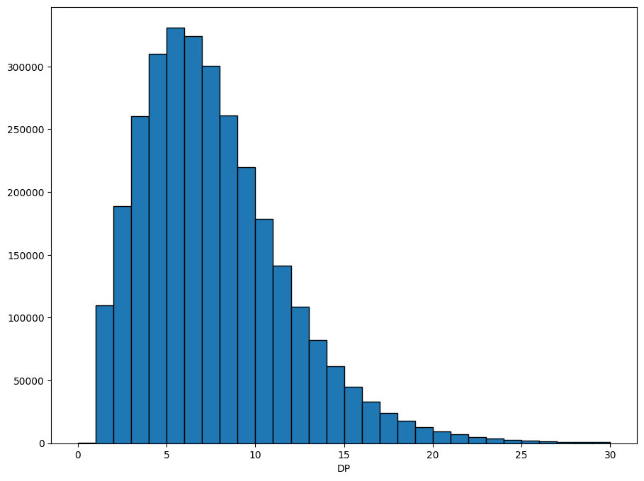
Often we want to plot the data, to get a feel for how it’s distributed. Xarray has some convenience functions for plotting, which we use here to show the distribution of the DP field.
dp = ds.call_DP.where(ds.call_DP >= 0) # filter out missing
dp.attrs["long_name"] = "DP"
xr.plot.hist(dp, range=(0, 30), bins=30, size=8, edgecolor="black");
Quality control#
QC is the process of filtering out poor quality data before running an analysis. This is usually an iterative process.
The sample_stats function in sgkit computes a collection of useful metrics for each sample and stores them in new variables. (The Hail equivalent is sample_qc.)
Here’s the dataset before running sample_stats.
ds
<xarray.Dataset>
Dimensions:               (samples: 284, variants: 10879, alleles: 2,
                           ploidy: 2, contigs: 84, filters: 1)
Dimensions without coordinates: samples, variants, alleles, ploidy, contigs,
                                filters
Data variables: (12/22)
    call_AD               (variants, samples, alleles) int32 dask.array<chunksize=(10000, 284, 2), meta=np.ndarray>
    call_DP               (variants, samples) int32 dask.array<chunksize=(10000, 284), meta=np.ndarray>
    call_GQ               (variants, samples) int32 dask.array<chunksize=(10000, 284), meta=np.ndarray>
    call_genotype         (variants, samples, ploidy) int8 dask.array<chunksize=(10000, 284, 2), meta=np.ndarray>
    call_genotype_mask    (variants, samples, ploidy) bool dask.array<chunksize=(10000, 284, 2), meta=np.ndarray>
    call_genotype_phased  (variants, samples) bool dask.array<chunksize=(10000, 284), meta=np.ndarray>
    ...                    ...
    variant_contig_name   (variants) int64 0 0 0 0 0 0 0 ... 22 22 22 22 22 22
    Population            (samples) object 'GBR' 'GBR' 'GBR' ... 'GIH' 'GIH'
    SuperPopulation       (samples) object 'EUR' 'EUR' 'EUR' ... 'SAS' 'SAS'
    isFemale              (samples) bool False True False ... False False True
    PurpleHair            (samples) bool False False False ... False True True
    CaffeineConsumption   (samples) int64 4 4 4 3 6 2 4 2 1 ... 5 6 4 6 4 6 5 5
Attributes: (7)- samples: 284
- variants: 10879
- alleles: 2
- ploidy: 2
- contigs: 84
- filters: 1
- call_AD(variants, samples, alleles)int32dask.array<chunksize=(10000, 284, 2), meta=np.ndarray>
Array Chunk Bytes 23.57 MiB 21.67 MiB Shape (10879, 284, 2) (10000, 284, 2) Count 2 Graph Layers 2 Chunks Type int32 numpy.ndarray - call_DP(variants, samples)int32dask.array<chunksize=(10000, 284), meta=np.ndarray>
Array Chunk Bytes 11.79 MiB 10.83 MiB Shape (10879, 284) (10000, 284) Count 2 Graph Layers 2 Chunks Type int32 numpy.ndarray - call_GQ(variants, samples)int32dask.array<chunksize=(10000, 284), meta=np.ndarray>
Array Chunk Bytes 11.79 MiB 10.83 MiB Shape (10879, 284) (10000, 284) Count 2 Graph Layers 2 Chunks Type int32 numpy.ndarray - call_genotype(variants, samples, ploidy)int8dask.array<chunksize=(10000, 284, 2), meta=np.ndarray>
- comment :
- Call genotype. Encoded as allele values (0 for the reference, 1 for the first allele, 2 for the second allele), -1 to indicate a missing value, or -2 to indicate a non allele in mixed ploidy datasets.
- mixed_ploidy :
- False
Array Chunk Bytes 5.89 MiB 5.42 MiB Shape (10879, 284, 2) (10000, 284, 2) Count 2 Graph Layers 2 Chunks Type int8 numpy.ndarray - call_genotype_mask(variants, samples, ploidy)booldask.array<chunksize=(10000, 284, 2), meta=np.ndarray>
- comment :
- A flag for each call indicating which values are missing.
Array Chunk Bytes 5.89 MiB 5.42 MiB Shape (10879, 284, 2) (10000, 284, 2) Count 2 Graph Layers 2 Chunks Type bool numpy.ndarray - call_genotype_phased(variants, samples)booldask.array<chunksize=(10000, 284), meta=np.ndarray>
- comment :
- A flag for each call indicating if it is phased or not. If omitted all calls are unphased.
Array Chunk Bytes 2.95 MiB 2.71 MiB Shape (10879, 284) (10000, 284) Count 2 Graph Layers 2 Chunks Type bool numpy.ndarray - contig_id(contigs)<U10dask.array<chunksize=(84,), meta=np.ndarray>
- comment :
- Contig identifiers.
Array Chunk Bytes 3.28 kiB 3.28 kiB Shape (84,) (84,) Count 2 Graph Layers 1 Chunks Type numpy.ndarray - contig_length(contigs)int64dask.array<chunksize=(84,), meta=np.ndarray>
Array Chunk Bytes 672 B 672 B Shape (84,) (84,) Count 2 Graph Layers 1 Chunks Type int64 numpy.ndarray - filter_id(filters)objectdask.array<chunksize=(1,), meta=np.ndarray>
Array Chunk Bytes 8 B 8 B Shape (1,) (1,) Count 2 Graph Layers 1 Chunks Type object numpy.ndarray - variant_allele(variants, alleles)objectdask.array<chunksize=(10000, 2), meta=np.ndarray>
- comment :
- The possible alleles for the variant.
Array Chunk Bytes 169.98 kiB 156.25 kiB Shape (10879, 2) (10000, 2) Count 2 Graph Layers 2 Chunks Type object numpy.ndarray - variant_contig(variants)int8dask.array<chunksize=(10000,), meta=np.ndarray>
- comment :
- Index corresponding to contig name for each variant. In some less common scenarios, this may also be equivalent to the contig names if the data generating process used contig names that were also integers.
Array Chunk Bytes 10.62 kiB 9.77 kiB Shape (10879,) (10000,) Count 2 Graph Layers 2 Chunks Type int8 numpy.ndarray - variant_filter(variants, filters)booldask.array<chunksize=(10000, 1), meta=np.ndarray>
Array Chunk Bytes 10.62 kiB 9.77 kiB Shape (10879, 1) (10000, 1) Count 2 Graph Layers 2 Chunks Type bool numpy.ndarray - variant_id(variants)objectdask.array<chunksize=(10000,), meta=np.ndarray>
- comment :
- The unique identifier of the variant.
Array Chunk Bytes 84.99 kiB 78.12 kiB Shape (10879,) (10000,) Count 2 Graph Layers 2 Chunks Type object numpy.ndarray - variant_id_mask(variants)booldask.array<chunksize=(10000,), meta=np.ndarray>
Array Chunk Bytes 10.62 kiB 9.77 kiB Shape (10879,) (10000,) Count 2 Graph Layers 2 Chunks Type bool numpy.ndarray - variant_position(variants)int32dask.array<chunksize=(10000,), meta=np.ndarray>
- comment :
- The reference position of the variant.
Array Chunk Bytes 42.50 kiB 39.06 kiB Shape (10879,) (10000,) Count 2 Graph Layers 2 Chunks Type int32 numpy.ndarray - variant_quality(variants)float32dask.array<chunksize=(10000,), meta=np.ndarray>
Array Chunk Bytes 42.50 kiB 39.06 kiB Shape (10879,) (10000,) Count 2 Graph Layers 2 Chunks Type float32 numpy.ndarray - variant_contig_name(variants)int640 0 0 0 0 0 0 ... 22 22 22 22 22 22
array([ 0, 0, 0, ..., 22, 22, 22])
- Population(samples)object'GBR' 'GBR' 'GBR' ... 'GIH' 'GIH'
array(['GBR', 'GBR', 'GBR', 'GBR', 'GBR', 'GBR', 'FIN', 'FIN', 'GBR', 'GBR', 'GBR', 'FIN', 'FIN', 'FIN', 'FIN', 'FIN', 'CHS', 'CHS', 'CHS', 'CHS', 'CHS', 'CHS', 'CHS', 'CHS', 'CHS', 'CHS', 'CHS', 'CHS', 'CHS', 'CHS', 'CHS', 'CHS', 'PUR', 'CDX', 'CDX', 'PUR', 'PUR', 'PUR', 'PUR', 'PUR', 'PUR', 'PUR', 'CLM', 'CLM', 'CLM', 'GBR', 'CLM', 'PUR', 'CLM', 'CLM', 'CLM', 'IBS', 'PEL', 'IBS', 'IBS', 'IBS', 'IBS', 'IBS', 'GBR', 'CDX', 'CDX', 'CDX', 'CDX', 'CDX', 'CDX', 'KHV', 'KHV', 'KHV', 'KHV', 'KHV', 'ACB', 'PEL', 'PEL', 'PEL', 'PEL', 'ACB', 'KHV', 'ACB', 'KHV', 'KHV', 'KHV', 'KHV', 'KHV', 'KHV', 'CDX', 'CDX', 'CDX', 'IBS', 'IBS', 'IBS', 'CDX', 'PEL', 'PEL', 'ACB', 'PEL', 'CDX', 'CDX', 'CDX', 'CDX', 'CDX', 'CDX', 'CDX', 'CDX', 'CDX', 'ACB', 'GWD', 'GWD', 'ACB', 'ACB', 'KHV', 'GWD', 'GWD', 'ACB', 'GWD', 'PJL', 'GWD', 'PJL', 'PJL', 'PJL', 'PJL', 'PJL', 'GWD', 'GWD', 'GWD', 'PJL', 'GWD', 'GWD', 'GWD', 'GWD', 'GWD', 'GWD', 'ESN', 'ESN', 'BEB', 'GWD', 'MSL', 'MSL', 'ESN', 'ESN', 'ESN', 'MSL', 'PJL', 'GWD', 'GWD', 'GWD', 'ESN', 'ESN', 'ESN', 'ESN', 'MSL', 'MSL', 'MSL', 'MSL', 'MSL', 'PJL', 'PJL', 'ESN', 'MSL', 'MSL', 'BEB', 'BEB', 'BEB', 'PJL', 'STU', 'STU', 'STU', 'ITU', 'STU', 'STU', 'BEB', 'BEB', 'BEB', 'STU', 'ITU', 'STU', 'BEB', 'BEB', 'STU', 'ITU', 'ITU', 'ITU', 'ITU', 'ITU', 'STU', 'BEB', 'BEB', 'ITU', 'STU', 'STU', 'ITU', 'CEU', 'CEU', 'CEU', 'CEU', 'CEU', 'CEU', 'CEU', 'CEU', 'CEU', 'CEU', 'YRI', 'CHB', 'CHB', 'CHB', 'CHB', 'CHB', 'CHB', 'CHB', 'CHB', 'CHB', 'CHB', 'CHB', 'YRI', 'YRI', 'YRI', 'YRI', 'YRI', 'JPT', 'JPT', 'JPT', 'JPT', 'JPT', 'JPT', 'JPT', 'JPT', 'JPT', 'JPT', 'JPT', 'YRI', 'YRI', 'YRI', 'YRI', 'YRI', 'LWK', 'LWK', 'LWK', 'LWK', 'LWK', 'LWK', 'LWK', 'LWK', 'LWK', 'LWK', 'LWK', 'LWK', 'LWK', 'LWK', 'LWK', 'MXL', 'MXL', 'MXL', 'MXL', 'MXL', 'ASW', 'MXL', 'MXL', 'MXL', 'MXL', 'MXL', 'ASW', 'ASW', 'TSI', 'TSI', 'TSI', 'TSI', 'TSI', 'TSI', 'TSI', 'TSI', 'TSI', 'TSI', 'GIH', 'GIH', 'GIH', 'GIH', 'GIH', 'GIH', 'GIH', 'GIH', 'GIH', 'GIH', 'GIH', 'GIH', 'GIH'], dtype=object) - SuperPopulation(samples)object'EUR' 'EUR' 'EUR' ... 'SAS' 'SAS'
array(['EUR', 'EUR', 'EUR', 'EUR', 'EUR', 'EUR', 'EUR', 'EUR', 'EUR', 'EUR', 'EUR', 'EUR', 'EUR', 'EUR', 'EUR', 'EUR', 'EAS', 'EAS', 'EAS', 'EAS', 'EAS', 'EAS', 'EAS', 'EAS', 'EAS', 'EAS', 'EAS', 'EAS', 'EAS', 'EAS', 'EAS', 'EAS', 'AMR', 'EAS', 'EAS', 'AMR', 'AMR', 'AMR', 'AMR', 'AMR', 'AMR', 'AMR', 'AMR', 'AMR', 'AMR', 'EUR', 'AMR', 'AMR', 'AMR', 'AMR', 'AMR', 'EUR', 'AMR', 'EUR', 'EUR', 'EUR', 'EUR', 'EUR', 'EUR', 'EAS', 'EAS', 'EAS', 'EAS', 'EAS', 'EAS', 'EAS', 'EAS', 'EAS', 'EAS', 'EAS', 'AFR', 'AMR', 'AMR', 'AMR', 'AMR', 'AFR', 'EAS', 'AFR', 'EAS', 'EAS', 'EAS', 'EAS', 'EAS', 'EAS', 'EAS', 'EAS', 'EAS', 'EUR', 'EUR', 'EUR', 'EAS', 'AMR', 'AMR', 'AFR', 'AMR', 'EAS', 'EAS', 'EAS', 'EAS', 'EAS', 'EAS', 'EAS', 'EAS', 'EAS', 'AFR', 'AFR', 'AFR', 'AFR', 'AFR', 'EAS', 'AFR', 'AFR', 'AFR', 'AFR', 'SAS', 'AFR', 'SAS', 'SAS', 'SAS', 'SAS', 'SAS', 'AFR', 'AFR', 'AFR', 'SAS', 'AFR', 'AFR', 'AFR', 'AFR', 'AFR', 'AFR', 'AFR', 'AFR', 'SAS', 'AFR', 'AFR', 'AFR', 'AFR', 'AFR', 'AFR', 'AFR', 'SAS', 'AFR', 'AFR', 'AFR', 'AFR', 'AFR', 'AFR', 'AFR', 'AFR', 'AFR', 'AFR', 'AFR', 'AFR', 'SAS', 'SAS', 'AFR', 'AFR', 'AFR', 'SAS', 'SAS', 'SAS', 'SAS', 'SAS', 'SAS', 'SAS', 'SAS', 'SAS', 'SAS', 'SAS', 'SAS', 'SAS', 'SAS', 'SAS', 'SAS', 'SAS', 'SAS', 'SAS', 'SAS', 'SAS', 'SAS', 'SAS', 'SAS', 'SAS', 'SAS', 'SAS', 'SAS', 'SAS', 'SAS', 'SAS', 'EUR', 'EUR', 'EUR', 'EUR', 'EUR', 'EUR', 'EUR', 'EUR', 'EUR', 'EUR', 'AFR', 'EAS', 'EAS', 'EAS', 'EAS', 'EAS', 'EAS', 'EAS', 'EAS', 'EAS', 'EAS', 'EAS', 'AFR', 'AFR', 'AFR', 'AFR', 'AFR', 'EAS', 'EAS', 'EAS', 'EAS', 'EAS', 'EAS', 'EAS', 'EAS', 'EAS', 'EAS', 'EAS', 'AFR', 'AFR', 'AFR', 'AFR', 'AFR', 'AFR', 'AFR', 'AFR', 'AFR', 'AFR', 'AFR', 'AFR', 'AFR', 'AFR', 'AFR', 'AFR', 'AFR', 'AFR', 'AFR', 'AFR', 'AMR', 'AMR', 'AMR', 'AMR', 'AMR', 'AFR', 'AMR', 'AMR', 'AMR', 'AMR', 'AMR', 'AFR', 'AFR', 'EUR', 'EUR', 'EUR', 'EUR', 'EUR', 'EUR', 'EUR', 'EUR', 'EUR', 'EUR', 'SAS', 'SAS', 'SAS', 'SAS', 'SAS', 'SAS', 'SAS', 'SAS', 'SAS', 'SAS', 'SAS', 'SAS', 'SAS'], dtype=object) - isFemale(samples)boolFalse True False ... False True
array([False, True, False, True, False, False, True, False, False, True, False, False, True, True, False, False, False, False, True, False, False, True, False, True, False, False, False, True, True, True, False, True, True, True, False, True, True, False, False, True, False, True, False, True, True, False, True, True, False, False, True, True, True, False, True, False, False, True, True, True, True, True, True, True, True, True, False, True, True, True, True, True, True, False, False, True, False, True, True, True, False, False, True, False, True, True, True, False, True, False, False, False, True, True, True, False, False, False, False, False, False, False, False, False, True, True, False, True, True, False, False, True, True, True, False, True, False, True, True, False, False, True, False, False, False, False, True, True, True, True, False, True, False, False, True, False, True, True, False, False, False, False, True, True, True, True, True, True, False, True, True, True, False, True, False, True, True, False, True, True, False, True, False, True, False, True, True, False, False, False, False, True, False, True, True, False, True, True, True, True, True, True, False, True, False, True, True, False, False, False, False, True, False, False, True, False, True, False, False, True, False, True, False, True, False, True, True, True, False, True, True, False, False, False, True, False, True, False, False, True, True, True, False, False, False, False, False, True, False, False, True, True, True, False, True, False, True, True, False, True, False, True, True, True, False, False, True, False, False, True, False, True, False, True, False, False, True, True, False, False, False, True, False, True, True, True, False, True, True, False, True, False, False, True, True, True, True, True, False, False, False, False, False, True]) - PurpleHair(samples)boolFalse False False ... True True
array([False, False, False, False, False, True, True, False, False, False, True, False, True, True, True, False, False, False, False, True, True, True, True, True, True, False, True, True, True, False, True, True, False, True, False, False, False, False, True, False, True, True, True, False, True, False, True, False, False, False, False, True, False, False, True, False, False, True, True, False, True, False, False, False, False, False, True, True, False, False, True, True, True, False, False, True, False, True, True, True, True, True, True, False, True, True, False, True, True, True, True, True, True, True, False, False, False, True, False, True, True, False, False, False, False, True, False, True, False, False, True, True, True, True, True, True, True, False, True, False, False, False, True, True, False, False, True, True, True, True, True, False, False, True, True, False, False, False, False, False, True, False, False, False, False, True, False, False, False, False, False, False, False, False, False, True, False, False, True, True, True, False, True, False, True, True, True, True, True, True, False, False, False, False, False, False, True, True, True, True, True, False, False, True, False, True, True, False, False, True, False, False, True, True, True, True, True, True, False, True, True, False, False, False, False, True, True, False, True, True, False, True, True, False, False, True, False, True, True, True, False, False, False, False, False, False, True, False, False, False, True, False, False, True, False, True, True, False, False, False, False, False, True, False, False, True, False, True, True, True, False, False, False, False, True, False, False, True, True, False, True, True, False, False, False, False, True, True, True, True, True, True, True, False, False, True, False, False, True, True, True, False, True, True]) - CaffeineConsumption(samples)int644 4 4 3 6 2 4 2 ... 5 6 4 6 4 6 5 5
array([4, 4, 4, 3, 6, 2, 4, 2, 1, 2, 0, 5, 4, 5, 4, 3, 6, 5, 5, 7, 5, 5,
       7, 5, 1, 5, 5, 5, 4, 4, 5, 5, 5, 6, 6, 4, 4, 6, 3, 3, 5, 4, 4, 5,
       5, 4, 6, 5, 4, 4, 5, 6, 3, 7, 5, 5, 6, 3, 2, 5, 5, 4, 6, 5, 6, 4,
       6, 7, 6, 7, 3, 5, 6, 5, 6, 4, 5, 4, 4, 5, 8, 3, 4, 4, 4, 7, 5, 4,
       2, 6, 7, 6, 5, 3, 3, 4, 5, 5, 5, 5, 6, 4, 5, 7, 2, 3, 3, 2, 3, 6,
       4, 2, 6, 5, 3, 4, 7, 6, 7, 6, 3, 4, 2, 2, 5, 6, 7, 8, 6, 2, 3, 2,
       0, 5, 7, 5, 1, 4, 3, 2, 4, 6, 5, 4, 4, 1, 5, 5, 3, 1, 1, 4, 3, 2,
       4, 2, 1, 3, 3, 4, 4, 5, 6, 5, 4, 5, 0, 4, 5, 4, 3, 3, 4, 4, 3, 5,
       6, 5, 3, 5, 4, 4, 6, 3, 5, 5, 4, 5, 3, 5, 4, 6, 5, 7, 5, 6, 6, 4,
       4, 5, 3, 5, 6, 5, 4, 3, 8, 2, 4, 4, 6, 8, 4, 3, 4, 3, 2, 5, 6, 6,
       4, 3, 5, 7, 4, 2, 5, 5, 6, 3, 2, 4, 4, 6, 5, 6, 5, 7, 2, 4, 2, 1,
       5, 3, 5, 3, 5, 2, 4, 9, 6, 4, 3, 4, 4, 6, 6, 7, 6, 6, 3, 4, 3, 6,
       6, 3, 4, 4, 2, 4, 6, 7, 4, 5, 4, 5, 5, 6, 4, 6, 4, 6, 5, 5])
- contig_lengths :
- [249250621, 243199373, 198022430, 191154276, 180915260, 171115067, 159138663, 146364022, 141213431, 135534747, 135006516, 133851895, 115169878, 107349540, 102531392, 90354753, 81195210, 78077248, 59128983, 63025520, 48129895, 51304566, 155270560, 59373566, 16569, 4262, 15008, 19913, 27386, 27682, 33824, 34474, 36148, 36422, 36651, 37175, 37498, 38154, 38502, 38914, 39786, 39929, 39939, 40103, 40531, 40652, 41001, 41933, 41934, 42152, 43341, 43523, 43691, 45867, 45941, 81310, 90085, 92689, 106433, 128374, 129120, 137718, 155397, 159169, 161147, 161802, 164239, 166566, 169874, 172149, 172294, 172545, 174588, 179198, 179693, 180455, 182896, 186858, 186861, 187035, 189789, 191469, 211173, 547496]
- contigs :
- ['1', '2', '3', '4', '5', '6', '7', '8', '9', '10', '11', '12', '13', '14', '15', '16', '17', '18', '19', '20', '21', '22', 'X', 'Y', 'MT', 'GL000207.1', 'GL000226.1', 'GL000229.1', 'GL000231.1', 'GL000210.1', 'GL000239.1', 'GL000235.1', 'GL000201.1', 'GL000247.1', 'GL000245.1', 'GL000197.1', 'GL000203.1', 'GL000246.1', 'GL000249.1', 'GL000196.1', 'GL000248.1', 'GL000244.1', 'GL000238.1', 'GL000202.1', 'GL000234.1', 'GL000232.1', 'GL000206.1', 'GL000240.1', 'GL000236.1', 'GL000241.1', 'GL000243.1', 'GL000242.1', 'GL000230.1', 'GL000237.1', 'GL000233.1', 'GL000204.1', 'GL000198.1', 'GL000208.1', 'GL000191.1', 'GL000227.1', 'GL000228.1', 'GL000214.1', 'GL000221.1', 'GL000209.1', 'GL000218.1', 'GL000220.1', 'GL000213.1', 'GL000211.1', 'GL000199.1', 'GL000217.1', 'GL000216.1', 'GL000215.1', 'GL000205.1', 'GL000219.1', 'GL000224.1', 'GL000223.1', 'GL000195.1', 'GL000212.1', 'GL000222.1', 'GL000200.1', 'GL000193.1', 'GL000194.1', 'GL000225.1', 'GL000192.1']
- filters :
- ['PASS']
- max_alt_alleles_seen :
- 1
- source :
- sgkit-0.6.1.dev2+gcc728043
- vcf_header :
- ##fileformat=VCFv4.2 ##FILTER=<ID=PASS,Description="All filters passed"> ##hailversion=0.2-29fbaeaf265e ##FORMAT=<ID=GT,Number=1,Type=String,Description=""> ##FORMAT=<ID=AD,Number=.,Type=Integer,Description=""> ##FORMAT=<ID=DP,Number=1,Type=Integer,Description=""> ##FORMAT=<ID=GQ,Number=1,Type=Integer,Description=""> ##FORMAT=<ID=PL,Number=.,Type=Integer,Description=""> ##INFO=<ID=AC,Number=.,Type=Integer,Description=""> ##INFO=<ID=AF,Number=.,Type=Float,Description=""> ##INFO=<ID=AN,Number=1,Type=Integer,Description=""> ##INFO=<ID=BaseQRankSum,Number=1,Type=Float,Description=""> ##INFO=<ID=ClippingRankSum,Number=1,Type=Float,Description=""> ##INFO=<ID=DP,Number=1,Type=Integer,Description=""> ##INFO=<ID=DS,Number=0,Type=Flag,Description=""> ##INFO=<ID=FS,Number=1,Type=Float,Description=""> ##INFO=<ID=HaplotypeScore,Number=1,Type=Float,Description=""> ##INFO=<ID=InbreedingCoeff,Number=1,Type=Float,Description=""> ##INFO=<ID=MLEAC,Number=.,Type=Integer,Description=""> ##INFO=<ID=MLEAF,Number=.,Type=Float,Description=""> ##INFO=<ID=MQ,Number=1,Type=Float,Description=""> ##INFO=<ID=MQ0,Number=1,Type=Integer,Description=""> ##INFO=<ID=MQRankSum,Number=1,Type=Float,Description=""> ##INFO=<ID=QD,Number=1,Type=Float,Description=""> ##INFO=<ID=ReadPosRankSum,Number=1,Type=Float,Description=""> ##INFO=<ID=set,Number=1,Type=String,Description=""> ##contig=<ID=1,length=249250621,assembly=GRCh37> ##contig=<ID=2,length=243199373,assembly=GRCh37> ##contig=<ID=3,length=198022430,assembly=GRCh37> ##contig=<ID=4,length=191154276,assembly=GRCh37> ##contig=<ID=5,length=180915260,assembly=GRCh37> ##contig=<ID=6,length=171115067,assembly=GRCh37> ##contig=<ID=7,length=159138663,assembly=GRCh37> ##contig=<ID=8,length=146364022,assembly=GRCh37> ##contig=<ID=9,length=141213431,assembly=GRCh37> ##contig=<ID=10,length=135534747,assembly=GRCh37> ##contig=<ID=11,length=135006516,assembly=GRCh37> ##contig=<ID=12,length=133851895,assembly=GRCh37> ##contig=<ID=13,length=115169878,assembly=GRCh37> ##contig=<ID=14,length=107349540,assembly=GRCh37> ##contig=<ID=15,length=102531392,assembly=GRCh37> ##contig=<ID=16,length=90354753,assembly=GRCh37> ##contig=<ID=17,length=81195210,assembly=GRCh37> ##contig=<ID=18,length=78077248,assembly=GRCh37> ##contig=<ID=19,length=59128983,assembly=GRCh37> ##contig=<ID=20,length=63025520,assembly=GRCh37> ##contig=<ID=21,length=48129895,assembly=GRCh37> ##contig=<ID=22,length=51304566,assembly=GRCh37> ##contig=<ID=X,length=155270560,assembly=GRCh37> ##contig=<ID=Y,length=59373566,assembly=GRCh37> ##contig=<ID=MT,length=16569,assembly=GRCh37> ##contig=<ID=GL000207.1,length=4262,assembly=GRCh37> ##contig=<ID=GL000226.1,length=15008,assembly=GRCh37> ##contig=<ID=GL000229.1,length=19913,assembly=GRCh37> ##contig=<ID=GL000231.1,length=27386,assembly=GRCh37> ##contig=<ID=GL000210.1,length=27682,assembly=GRCh37> ##contig=<ID=GL000239.1,length=33824,assembly=GRCh37> ##contig=<ID=GL000235.1,length=34474,assembly=GRCh37> ##contig=<ID=GL000201.1,length=36148,assembly=GRCh37> ##contig=<ID=GL000247.1,length=36422,assembly=GRCh37> ##contig=<ID=GL000245.1,length=36651,assembly=GRCh37> ##contig=<ID=GL000197.1,length=37175,assembly=GRCh37> ##contig=<ID=GL000203.1,length=37498,assembly=GRCh37> ##contig=<ID=GL000246.1,length=38154,assembly=GRCh37> ##contig=<ID=GL000249.1,length=38502,assembly=GRCh37> ##contig=<ID=GL000196.1,length=38914,assembly=GRCh37> ##contig=<ID=GL000248.1,length=39786,assembly=GRCh37> ##contig=<ID=GL000244.1,length=39929,assembly=GRCh37> ##contig=<ID=GL000238.1,length=39939,assembly=GRCh37> ##contig=<ID=GL000202.1,length=40103,assembly=GRCh37> ##contig=<ID=GL000234.1,length=40531,assembly=GRCh37> ##contig=<ID=GL000232.1,length=40652,assembly=GRCh37> ##contig=<ID=GL000206.1,length=41001,assembly=GRCh37> ##contig=<ID=GL000240.1,length=41933,assembly=GRCh37> ##contig=<ID=GL000236.1,length=41934,assembly=GRCh37> ##contig=<ID=GL000241.1,length=42152,assembly=GRCh37> ##contig=<ID=GL000243.1,length=43341,assembly=GRCh37> ##contig=<ID=GL000242.1,length=43523,assembly=GRCh37> ##contig=<ID=GL000230.1,length=43691,assembly=GRCh37> ##contig=<ID=GL000237.1,length=45867,assembly=GRCh37> ##contig=<ID=GL000233.1,length=45941,assembly=GRCh37> ##contig=<ID=GL000204.1,length=81310,assembly=GRCh37> ##contig=<ID=GL000198.1,length=90085,assembly=GRCh37> ##contig=<ID=GL000208.1,length=92689,assembly=GRCh37> ##contig=<ID=GL000191.1,length=106433,assembly=GRCh37> ##contig=<ID=GL000227.1,length=128374,assembly=GRCh37> ##contig=<ID=GL000228.1,length=129120,assembly=GRCh37> ##contig=<ID=GL000214.1,length=137718,assembly=GRCh37> ##contig=<ID=GL000221.1,length=155397,assembly=GRCh37> ##contig=<ID=GL000209.1,length=159169,assembly=GRCh37> ##contig=<ID=GL000218.1,length=161147,assembly=GRCh37> ##contig=<ID=GL000220.1,length=161802,assembly=GRCh37> ##contig=<ID=GL000213.1,length=164239,assembly=GRCh37> ##contig=<ID=GL000211.1,length=166566,assembly=GRCh37> ##contig=<ID=GL000199.1,length=169874,assembly=GRCh37> ##contig=<ID=GL000217.1,length=172149,assembly=GRCh37> ##contig=<ID=GL000216.1,length=172294,assembly=GRCh37> ##contig=<ID=GL000215.1,length=172545,assembly=GRCh37> ##contig=<ID=GL000205.1,length=174588,assembly=GRCh37> ##contig=<ID=GL000219.1,length=179198,assembly=GRCh37> ##contig=<ID=GL000224.1,length=179693,assembly=GRCh37> ##contig=<ID=GL000223.1,length=180455,assembly=GRCh37> ##contig=<ID=GL000195.1,length=182896,assembly=GRCh37> ##contig=<ID=GL000212.1,length=186858,assembly=GRCh37> ##contig=<ID=GL000222.1,length=186861,assembly=GRCh37> ##contig=<ID=GL000200.1,length=187035,assembly=GRCh37> ##contig=<ID=GL000193.1,length=189789,assembly=GRCh37> ##contig=<ID=GL000194.1,length=191469,assembly=GRCh37> ##contig=<ID=GL000225.1,length=211173,assembly=GRCh37> ##contig=<ID=GL000192.1,length=547496,assembly=GRCh37> #CHROM POS ID REF ALT QUAL FILTER INFO FORMAT HG00096 HG00099 HG00105 HG00118 HG00129 HG00148 HG00177 HG00182 HG00242 HG00254 HG00265 HG00271 HG00274 HG00332 HG00335 HG00369 HG00421 HG00436 HG00452 HG00472 HG00530 HG00534 HG00583 HG00590 HG00598 HG00607 HG00619 HG00623 HG00657 HG00663 HG00704 HG00705 HG00733 HG00864 HG00881 HG01052 HG01070 HG01075 HG01164 HG01174 HG01241 HG01248 HG01256 HG01275 HG01284 HG01334 HG01348 HG01396 HG01443 HG01491 HG01498 HG01537 HG01572 HG01606 HG01623 HG01630 HG01783 HG01784 HG01790 HG01799 HG01801 HG01806 HG01812 HG01813 HG01817 HG01848 HG01849 HG01857 HG01863 HG01874 HG01915 HG01924 HG01965 HG01970 HG01991 HG02010 HG02020 HG02054 HG02086 HG02087 HG02116 HG02122 HG02130 HG02131 HG02152 HG02154 HG02165 HG02224 HG02232 HG02236 HG02250 HG02259 HG02298 HG02318 HG02345 HG02351 HG02363 HG02373 HG02383 HG02384 HG02386 HG02388 HG02389 HG02397 HG02419 HG02462 HG02464 HG02497 HG02511 HG02521 HG02561 HG02574 HG02580 HG02595 HG02603 HG02629 HG02651 HG02682 HG02688 HG02690 HG02699 HG02760 HG02768 HG02771 HG02792 HG02798 HG02811 HG02814 HG02840 HG02870 HG02881 HG02970 HG02973 HG03009 HG03046 HG03074 HG03091 HG03105 HG03127 HG03193 HG03224 HG03237 HG03241 HG03247 HG03259 HG03267 HG03354 HG03366 HG03367 HG03380 HG03419 HG03449 HG03451 HG03458 HG03490 HG03491 HG03511 HG03556 HG03563 HG03598 HG03603 HG03607 HG03636 HG03684 HG03686 HG03690 HG03731 HG03740 HG03755 HG03800 HG03815 HG03832 HG03850 HG03873 HG03897 HG03905 HG03937 HG03948 HG03973 HG04054 HG04059 HG04063 HG04096 HG04099 HG04140 HG04171 HG04209 HG04210 HG04229 HG04239 NA07347 NA11918 NA11919 NA12045 NA12273 NA12342 NA12414 NA12546 NA12760 NA12878 NA18516 NA18525 NA18534 NA18541 NA18557 NA18565 NA18616 NA18619 NA18623 NA18630 NA18631 NA18740 NA18853 NA18865 NA18873 NA18874 NA18916 NA18960 NA18966 NA18975 NA18976 NA18978 NA18990 NA19060 NA19063 NA19076 NA19086 NA19087 NA19096 NA19113 NA19118 NA19185 NA19209 NA19311 NA19314 NA19317 NA19321 NA19379 NA19384 NA19390 NA19397 NA19399 NA19404 NA19446 NA19448 NA19455 NA19456 NA19466 NA19655 NA19657 NA19670 NA19678 NA19679 NA19701 NA19720 NA19756 NA19761 NA19764 NA19786 NA20318 NA20351 NA20517 NA20518 NA20529 NA20587 NA20757 NA20798 NA20799 NA20800 NA20810 NA20826 NA20858 NA20864 NA20869 NA20877 NA20888 NA20910 NA21101 NA21113 NA21114 NA21116 NA21118 NA21133 NA21143
- vcf_zarr_version :
- 0.2
We can see the new variables (with names beginning sample_) after we run sample_stats:
ds = sg.sample_stats(ds)
ds
<xarray.Dataset>
Dimensions:               (samples: 284, variants: 10879, alleles: 2,
                           ploidy: 2, contigs: 84, filters: 1)
Dimensions without coordinates: samples, variants, alleles, ploidy, contigs,
                                filters
Data variables: (12/28)
    sample_n_called       (samples) int64 dask.array<chunksize=(284,), meta=np.ndarray>
    sample_call_rate      (samples) float64 dask.array<chunksize=(284,), meta=np.ndarray>
    sample_n_het          (samples) int64 dask.array<chunksize=(284,), meta=np.ndarray>
    sample_n_hom_ref      (samples) int64 dask.array<chunksize=(284,), meta=np.ndarray>
    sample_n_hom_alt      (samples) int64 dask.array<chunksize=(284,), meta=np.ndarray>
    sample_n_non_ref      (samples) int64 dask.array<chunksize=(284,), meta=np.ndarray>
    ...                    ...
    variant_contig_name   (variants) int64 0 0 0 0 0 0 0 ... 22 22 22 22 22 22
    Population            (samples) object 'GBR' 'GBR' 'GBR' ... 'GIH' 'GIH'
    SuperPopulation       (samples) object 'EUR' 'EUR' 'EUR' ... 'SAS' 'SAS'
    isFemale              (samples) bool False True False ... False False True
    PurpleHair            (samples) bool False False False ... False True True
    CaffeineConsumption   (samples) int64 4 4 4 3 6 2 4 2 1 ... 5 6 4 6 4 6 5 5
Attributes: (7)- samples: 284
- variants: 10879
- alleles: 2
- ploidy: 2
- contigs: 84
- filters: 1
- sample_n_called(samples)int64dask.array<chunksize=(284,), meta=np.ndarray>
- comment :
- The number of variants with called genotypes.
Array Chunk Bytes 2.22 kiB 2.22 kiB Shape (284,) (284,) Count 7 Graph Layers 1 Chunks Type int64 numpy.ndarray - sample_call_rate(samples)float64dask.array<chunksize=(284,), meta=np.ndarray>
- comment :
- The fraction of variants with called genotypes.
Array Chunk Bytes 2.22 kiB 2.22 kiB Shape (284,) (284,) Count 8 Graph Layers 1 Chunks Type float64 numpy.ndarray - sample_n_het(samples)int64dask.array<chunksize=(284,), meta=np.ndarray>
- comment :
- The number of variants with heterozygous calls.
Array Chunk Bytes 2.22 kiB 2.22 kiB Shape (284,) (284,) Count 22 Graph Layers 1 Chunks Type int64 numpy.ndarray - sample_n_hom_ref(samples)int64dask.array<chunksize=(284,), meta=np.ndarray>
- comment :
- The number of variants with homozygous reference calls.
Array Chunk Bytes 2.22 kiB 2.22 kiB Shape (284,) (284,) Count 12 Graph Layers 1 Chunks Type int64 numpy.ndarray - sample_n_hom_alt(samples)int64dask.array<chunksize=(284,), meta=np.ndarray>
- comment :
- The number of variants with homozygous alternate calls.
Array Chunk Bytes 2.22 kiB 2.22 kiB Shape (284,) (284,) Count 17 Graph Layers 1 Chunks Type int64 numpy.ndarray - sample_n_non_ref(samples)int64dask.array<chunksize=(284,), meta=np.ndarray>
- comment :
- The number of variants that are not homozygous reference calls.
Array Chunk Bytes 2.22 kiB 2.22 kiB Shape (284,) (284,) Count 12 Graph Layers 1 Chunks Type int64 numpy.ndarray - call_AD(variants, samples, alleles)int32dask.array<chunksize=(10000, 284, 2), meta=np.ndarray>
Array Chunk Bytes 23.57 MiB 21.67 MiB Shape (10879, 284, 2) (10000, 284, 2) Count 2 Graph Layers 2 Chunks Type int32 numpy.ndarray - call_DP(variants, samples)int32dask.array<chunksize=(10000, 284), meta=np.ndarray>
Array Chunk Bytes 11.79 MiB 10.83 MiB Shape (10879, 284) (10000, 284) Count 2 Graph Layers 2 Chunks Type int32 numpy.ndarray - call_GQ(variants, samples)int32dask.array<chunksize=(10000, 284), meta=np.ndarray>
Array Chunk Bytes 11.79 MiB 10.83 MiB Shape (10879, 284) (10000, 284) Count 2 Graph Layers 2 Chunks Type int32 numpy.ndarray - call_genotype(variants, samples, ploidy)int8dask.array<chunksize=(10000, 284, 2), meta=np.ndarray>
- comment :
- Call genotype. Encoded as allele values (0 for the reference, 1 for the first allele, 2 for the second allele), -1 to indicate a missing value, or -2 to indicate a non allele in mixed ploidy datasets.
- mixed_ploidy :
- False
Array Chunk Bytes 5.89 MiB 5.42 MiB Shape (10879, 284, 2) (10000, 284, 2) Count 2 Graph Layers 2 Chunks Type int8 numpy.ndarray - call_genotype_mask(variants, samples, ploidy)booldask.array<chunksize=(10000, 284, 2), meta=np.ndarray>
- comment :
- A flag for each call indicating which values are missing.
Array Chunk Bytes 5.89 MiB 5.42 MiB Shape (10879, 284, 2) (10000, 284, 2) Count 2 Graph Layers 2 Chunks Type bool numpy.ndarray - call_genotype_phased(variants, samples)booldask.array<chunksize=(10000, 284), meta=np.ndarray>
- comment :
- A flag for each call indicating if it is phased or not. If omitted all calls are unphased.
Array Chunk Bytes 2.95 MiB 2.71 MiB Shape (10879, 284) (10000, 284) Count 2 Graph Layers 2 Chunks Type bool numpy.ndarray - contig_id(contigs)<U10dask.array<chunksize=(84,), meta=np.ndarray>
- comment :
- Contig identifiers.
Array Chunk Bytes 3.28 kiB 3.28 kiB Shape (84,) (84,) Count 2 Graph Layers 1 Chunks Type numpy.ndarray - contig_length(contigs)int64dask.array<chunksize=(84,), meta=np.ndarray>
Array Chunk Bytes 672 B 672 B Shape (84,) (84,) Count 2 Graph Layers 1 Chunks Type int64 numpy.ndarray - filter_id(filters)objectdask.array<chunksize=(1,), meta=np.ndarray>
Array Chunk Bytes 8 B 8 B Shape (1,) (1,) Count 2 Graph Layers 1 Chunks Type object numpy.ndarray - variant_allele(variants, alleles)objectdask.array<chunksize=(10000, 2), meta=np.ndarray>
- comment :
- The possible alleles for the variant.
Array Chunk Bytes 169.98 kiB 156.25 kiB Shape (10879, 2) (10000, 2) Count 2 Graph Layers 2 Chunks Type object numpy.ndarray - variant_contig(variants)int8dask.array<chunksize=(10000,), meta=np.ndarray>
- comment :
- Index corresponding to contig name for each variant. In some less common scenarios, this may also be equivalent to the contig names if the data generating process used contig names that were also integers.
Array Chunk Bytes 10.62 kiB 9.77 kiB Shape (10879,) (10000,) Count 2 Graph Layers 2 Chunks Type int8 numpy.ndarray - variant_filter(variants, filters)booldask.array<chunksize=(10000, 1), meta=np.ndarray>
Array Chunk Bytes 10.62 kiB 9.77 kiB Shape (10879, 1) (10000, 1) Count 2 Graph Layers 2 Chunks Type bool numpy.ndarray - variant_id(variants)objectdask.array<chunksize=(10000,), meta=np.ndarray>
- comment :
- The unique identifier of the variant.
Array Chunk Bytes 84.99 kiB 78.12 kiB Shape (10879,) (10000,) Count 2 Graph Layers 2 Chunks Type object numpy.ndarray - variant_id_mask(variants)booldask.array<chunksize=(10000,), meta=np.ndarray>
Array Chunk Bytes 10.62 kiB 9.77 kiB Shape (10879,) (10000,) Count 2 Graph Layers 2 Chunks Type bool numpy.ndarray - variant_position(variants)int32dask.array<chunksize=(10000,), meta=np.ndarray>
- comment :
- The reference position of the variant.
Array Chunk Bytes 42.50 kiB 39.06 kiB Shape (10879,) (10000,) Count 2 Graph Layers 2 Chunks Type int32 numpy.ndarray - variant_quality(variants)float32dask.array<chunksize=(10000,), meta=np.ndarray>
Array Chunk Bytes 42.50 kiB 39.06 kiB Shape (10879,) (10000,) Count 2 Graph Layers 2 Chunks Type float32 numpy.ndarray - variant_contig_name(variants)int640 0 0 0 0 0 0 ... 22 22 22 22 22 22
array([ 0, 0, 0, ..., 22, 22, 22])
- Population(samples)object'GBR' 'GBR' 'GBR' ... 'GIH' 'GIH'
array(['GBR', 'GBR', 'GBR', 'GBR', 'GBR', 'GBR', 'FIN', 'FIN', 'GBR', 'GBR', 'GBR', 'FIN', 'FIN', 'FIN', 'FIN', 'FIN', 'CHS', 'CHS', 'CHS', 'CHS', 'CHS', 'CHS', 'CHS', 'CHS', 'CHS', 'CHS', 'CHS', 'CHS', 'CHS', 'CHS', 'CHS', 'CHS', 'PUR', 'CDX', 'CDX', 'PUR', 'PUR', 'PUR', 'PUR', 'PUR', 'PUR', 'PUR', 'CLM', 'CLM', 'CLM', 'GBR', 'CLM', 'PUR', 'CLM', 'CLM', 'CLM', 'IBS', 'PEL', 'IBS', 'IBS', 'IBS', 'IBS', 'IBS', 'GBR', 'CDX', 'CDX', 'CDX', 'CDX', 'CDX', 'CDX', 'KHV', 'KHV', 'KHV', 'KHV', 'KHV', 'ACB', 'PEL', 'PEL', 'PEL', 'PEL', 'ACB', 'KHV', 'ACB', 'KHV', 'KHV', 'KHV', 'KHV', 'KHV', 'KHV', 'CDX', 'CDX', 'CDX', 'IBS', 'IBS', 'IBS', 'CDX', 'PEL', 'PEL', 'ACB', 'PEL', 'CDX', 'CDX', 'CDX', 'CDX', 'CDX', 'CDX', 'CDX', 'CDX', 'CDX', 'ACB', 'GWD', 'GWD', 'ACB', 'ACB', 'KHV', 'GWD', 'GWD', 'ACB', 'GWD', 'PJL', 'GWD', 'PJL', 'PJL', 'PJL', 'PJL', 'PJL', 'GWD', 'GWD', 'GWD', 'PJL', 'GWD', 'GWD', 'GWD', 'GWD', 'GWD', 'GWD', 'ESN', 'ESN', 'BEB', 'GWD', 'MSL', 'MSL', 'ESN', 'ESN', 'ESN', 'MSL', 'PJL', 'GWD', 'GWD', 'GWD', 'ESN', 'ESN', 'ESN', 'ESN', 'MSL', 'MSL', 'MSL', 'MSL', 'MSL', 'PJL', 'PJL', 'ESN', 'MSL', 'MSL', 'BEB', 'BEB', 'BEB', 'PJL', 'STU', 'STU', 'STU', 'ITU', 'STU', 'STU', 'BEB', 'BEB', 'BEB', 'STU', 'ITU', 'STU', 'BEB', 'BEB', 'STU', 'ITU', 'ITU', 'ITU', 'ITU', 'ITU', 'STU', 'BEB', 'BEB', 'ITU', 'STU', 'STU', 'ITU', 'CEU', 'CEU', 'CEU', 'CEU', 'CEU', 'CEU', 'CEU', 'CEU', 'CEU', 'CEU', 'YRI', 'CHB', 'CHB', 'CHB', 'CHB', 'CHB', 'CHB', 'CHB', 'CHB', 'CHB', 'CHB', 'CHB', 'YRI', 'YRI', 'YRI', 'YRI', 'YRI', 'JPT', 'JPT', 'JPT', 'JPT', 'JPT', 'JPT', 'JPT', 'JPT', 'JPT', 'JPT', 'JPT', 'YRI', 'YRI', 'YRI', 'YRI', 'YRI', 'LWK', 'LWK', 'LWK', 'LWK', 'LWK', 'LWK', 'LWK', 'LWK', 'LWK', 'LWK', 'LWK', 'LWK', 'LWK', 'LWK', 'LWK', 'MXL', 'MXL', 'MXL', 'MXL', 'MXL', 'ASW', 'MXL', 'MXL', 'MXL', 'MXL', 'MXL', 'ASW', 'ASW', 'TSI', 'TSI', 'TSI', 'TSI', 'TSI', 'TSI', 'TSI', 'TSI', 'TSI', 'TSI', 'GIH', 'GIH', 'GIH', 'GIH', 'GIH', 'GIH', 'GIH', 'GIH', 'GIH', 'GIH', 'GIH', 'GIH', 'GIH'], dtype=object) - SuperPopulation(samples)object'EUR' 'EUR' 'EUR' ... 'SAS' 'SAS'
array(['EUR', 'EUR', 'EUR', 'EUR', 'EUR', 'EUR', 'EUR', 'EUR', 'EUR', 'EUR', 'EUR', 'EUR', 'EUR', 'EUR', 'EUR', 'EUR', 'EAS', 'EAS', 'EAS', 'EAS', 'EAS', 'EAS', 'EAS', 'EAS', 'EAS', 'EAS', 'EAS', 'EAS', 'EAS', 'EAS', 'EAS', 'EAS', 'AMR', 'EAS', 'EAS', 'AMR', 'AMR', 'AMR', 'AMR', 'AMR', 'AMR', 'AMR', 'AMR', 'AMR', 'AMR', 'EUR', 'AMR', 'AMR', 'AMR', 'AMR', 'AMR', 'EUR', 'AMR', 'EUR', 'EUR', 'EUR', 'EUR', 'EUR', 'EUR', 'EAS', 'EAS', 'EAS', 'EAS', 'EAS', 'EAS', 'EAS', 'EAS', 'EAS', 'EAS', 'EAS', 'AFR', 'AMR', 'AMR', 'AMR', 'AMR', 'AFR', 'EAS', 'AFR', 'EAS', 'EAS', 'EAS', 'EAS', 'EAS', 'EAS', 'EAS', 'EAS', 'EAS', 'EUR', 'EUR', 'EUR', 'EAS', 'AMR', 'AMR', 'AFR', 'AMR', 'EAS', 'EAS', 'EAS', 'EAS', 'EAS', 'EAS', 'EAS', 'EAS', 'EAS', 'AFR', 'AFR', 'AFR', 'AFR', 'AFR', 'EAS', 'AFR', 'AFR', 'AFR', 'AFR', 'SAS', 'AFR', 'SAS', 'SAS', 'SAS', 'SAS', 'SAS', 'AFR', 'AFR', 'AFR', 'SAS', 'AFR', 'AFR', 'AFR', 'AFR', 'AFR', 'AFR', 'AFR', 'AFR', 'SAS', 'AFR', 'AFR', 'AFR', 'AFR', 'AFR', 'AFR', 'AFR', 'SAS', 'AFR', 'AFR', 'AFR', 'AFR', 'AFR', 'AFR', 'AFR', 'AFR', 'AFR', 'AFR', 'AFR', 'AFR', 'SAS', 'SAS', 'AFR', 'AFR', 'AFR', 'SAS', 'SAS', 'SAS', 'SAS', 'SAS', 'SAS', 'SAS', 'SAS', 'SAS', 'SAS', 'SAS', 'SAS', 'SAS', 'SAS', 'SAS', 'SAS', 'SAS', 'SAS', 'SAS', 'SAS', 'SAS', 'SAS', 'SAS', 'SAS', 'SAS', 'SAS', 'SAS', 'SAS', 'SAS', 'SAS', 'SAS', 'EUR', 'EUR', 'EUR', 'EUR', 'EUR', 'EUR', 'EUR', 'EUR', 'EUR', 'EUR', 'AFR', 'EAS', 'EAS', 'EAS', 'EAS', 'EAS', 'EAS', 'EAS', 'EAS', 'EAS', 'EAS', 'EAS', 'AFR', 'AFR', 'AFR', 'AFR', 'AFR', 'EAS', 'EAS', 'EAS', 'EAS', 'EAS', 'EAS', 'EAS', 'EAS', 'EAS', 'EAS', 'EAS', 'AFR', 'AFR', 'AFR', 'AFR', 'AFR', 'AFR', 'AFR', 'AFR', 'AFR', 'AFR', 'AFR', 'AFR', 'AFR', 'AFR', 'AFR', 'AFR', 'AFR', 'AFR', 'AFR', 'AFR', 'AMR', 'AMR', 'AMR', 'AMR', 'AMR', 'AFR', 'AMR', 'AMR', 'AMR', 'AMR', 'AMR', 'AFR', 'AFR', 'EUR', 'EUR', 'EUR', 'EUR', 'EUR', 'EUR', 'EUR', 'EUR', 'EUR', 'EUR', 'SAS', 'SAS', 'SAS', 'SAS', 'SAS', 'SAS', 'SAS', 'SAS', 'SAS', 'SAS', 'SAS', 'SAS', 'SAS'], dtype=object) - isFemale(samples)boolFalse True False ... False True
array([False, True, False, True, False, False, True, False, False, True, False, False, True, True, False, False, False, False, True, False, False, True, False, True, False, False, False, True, True, True, False, True, True, True, False, True, True, False, False, True, False, True, False, True, True, False, True, True, False, False, True, True, True, False, True, False, False, True, True, True, True, True, True, True, True, True, False, True, True, True, True, True, True, False, False, True, False, True, True, True, False, False, True, False, True, True, True, False, True, False, False, False, True, True, True, False, False, False, False, False, False, False, False, False, True, True, False, True, True, False, False, True, True, True, False, True, False, True, True, False, False, True, False, False, False, False, True, True, True, True, False, True, False, False, True, False, True, True, False, False, False, False, True, True, True, True, True, True, False, True, True, True, False, True, False, True, True, False, True, True, False, True, False, True, False, True, True, False, False, False, False, True, False, True, True, False, True, True, True, True, True, True, False, True, False, True, True, False, False, False, False, True, False, False, True, False, True, False, False, True, False, True, False, True, False, True, True, True, False, True, True, False, False, False, True, False, True, False, False, True, True, True, False, False, False, False, False, True, False, False, True, True, True, False, True, False, True, True, False, True, False, True, True, True, False, False, True, False, False, True, False, True, False, True, False, False, True, True, False, False, False, True, False, True, True, True, False, True, True, False, True, False, False, True, True, True, True, True, False, False, False, False, False, True]) - PurpleHair(samples)boolFalse False False ... True True
array([False, False, False, False, False, True, True, False, False, False, True, False, True, True, True, False, False, False, False, True, True, True, True, True, True, False, True, True, True, False, True, True, False, True, False, False, False, False, True, False, True, True, True, False, True, False, True, False, False, False, False, True, False, False, True, False, False, True, True, False, True, False, False, False, False, False, True, True, False, False, True, True, True, False, False, True, False, True, True, True, True, True, True, False, True, True, False, True, True, True, True, True, True, True, False, False, False, True, False, True, True, False, False, False, False, True, False, True, False, False, True, True, True, True, True, True, True, False, True, False, False, False, True, True, False, False, True, True, True, True, True, False, False, True, True, False, False, False, False, False, True, False, False, False, False, True, False, False, False, False, False, False, False, False, False, True, False, False, True, True, True, False, True, False, True, True, True, True, True, True, False, False, False, False, False, False, True, True, True, True, True, False, False, True, False, True, True, False, False, True, False, False, True, True, True, True, True, True, False, True, True, False, False, False, False, True, True, False, True, True, False, True, True, False, False, True, False, True, True, True, False, False, False, False, False, False, True, False, False, False, True, False, False, True, False, True, True, False, False, False, False, False, True, False, False, True, False, True, True, True, False, False, False, False, True, False, False, True, True, False, True, True, False, False, False, False, True, True, True, True, True, True, True, False, False, True, False, False, True, True, True, False, True, True]) - CaffeineConsumption(samples)int644 4 4 3 6 2 4 2 ... 5 6 4 6 4 6 5 5
array([4, 4, 4, 3, 6, 2, 4, 2, 1, 2, 0, 5, 4, 5, 4, 3, 6, 5, 5, 7, 5, 5,
       7, 5, 1, 5, 5, 5, 4, 4, 5, 5, 5, 6, 6, 4, 4, 6, 3, 3, 5, 4, 4, 5,
       5, 4, 6, 5, 4, 4, 5, 6, 3, 7, 5, 5, 6, 3, 2, 5, 5, 4, 6, 5, 6, 4,
       6, 7, 6, 7, 3, 5, 6, 5, 6, 4, 5, 4, 4, 5, 8, 3, 4, 4, 4, 7, 5, 4,
       2, 6, 7, 6, 5, 3, 3, 4, 5, 5, 5, 5, 6, 4, 5, 7, 2, 3, 3, 2, 3, 6,
       4, 2, 6, 5, 3, 4, 7, 6, 7, 6, 3, 4, 2, 2, 5, 6, 7, 8, 6, 2, 3, 2,
       0, 5, 7, 5, 1, 4, 3, 2, 4, 6, 5, 4, 4, 1, 5, 5, 3, 1, 1, 4, 3, 2,
       4, 2, 1, 3, 3, 4, 4, 5, 6, 5, 4, 5, 0, 4, 5, 4, 3, 3, 4, 4, 3, 5,
       6, 5, 3, 5, 4, 4, 6, 3, 5, 5, 4, 5, 3, 5, 4, 6, 5, 7, 5, 6, 6, 4,
       4, 5, 3, 5, 6, 5, 4, 3, 8, 2, 4, 4, 6, 8, 4, 3, 4, 3, 2, 5, 6, 6,
       4, 3, 5, 7, 4, 2, 5, 5, 6, 3, 2, 4, 4, 6, 5, 6, 5, 7, 2, 4, 2, 1,
       5, 3, 5, 3, 5, 2, 4, 9, 6, 4, 3, 4, 4, 6, 6, 7, 6, 6, 3, 4, 3, 6,
       6, 3, 4, 4, 2, 4, 6, 7, 4, 5, 4, 5, 5, 6, 4, 6, 4, 6, 5, 5])
- contig_lengths :
- [249250621, 243199373, 198022430, 191154276, 180915260, 171115067, 159138663, 146364022, 141213431, 135534747, 135006516, 133851895, 115169878, 107349540, 102531392, 90354753, 81195210, 78077248, 59128983, 63025520, 48129895, 51304566, 155270560, 59373566, 16569, 4262, 15008, 19913, 27386, 27682, 33824, 34474, 36148, 36422, 36651, 37175, 37498, 38154, 38502, 38914, 39786, 39929, 39939, 40103, 40531, 40652, 41001, 41933, 41934, 42152, 43341, 43523, 43691, 45867, 45941, 81310, 90085, 92689, 106433, 128374, 129120, 137718, 155397, 159169, 161147, 161802, 164239, 166566, 169874, 172149, 172294, 172545, 174588, 179198, 179693, 180455, 182896, 186858, 186861, 187035, 189789, 191469, 211173, 547496]
- contigs :
- ['1', '2', '3', '4', '5', '6', '7', '8', '9', '10', '11', '12', '13', '14', '15', '16', '17', '18', '19', '20', '21', '22', 'X', 'Y', 'MT', 'GL000207.1', 'GL000226.1', 'GL000229.1', 'GL000231.1', 'GL000210.1', 'GL000239.1', 'GL000235.1', 'GL000201.1', 'GL000247.1', 'GL000245.1', 'GL000197.1', 'GL000203.1', 'GL000246.1', 'GL000249.1', 'GL000196.1', 'GL000248.1', 'GL000244.1', 'GL000238.1', 'GL000202.1', 'GL000234.1', 'GL000232.1', 'GL000206.1', 'GL000240.1', 'GL000236.1', 'GL000241.1', 'GL000243.1', 'GL000242.1', 'GL000230.1', 'GL000237.1', 'GL000233.1', 'GL000204.1', 'GL000198.1', 'GL000208.1', 'GL000191.1', 'GL000227.1', 'GL000228.1', 'GL000214.1', 'GL000221.1', 'GL000209.1', 'GL000218.1', 'GL000220.1', 'GL000213.1', 'GL000211.1', 'GL000199.1', 'GL000217.1', 'GL000216.1', 'GL000215.1', 'GL000205.1', 'GL000219.1', 'GL000224.1', 'GL000223.1', 'GL000195.1', 'GL000212.1', 'GL000222.1', 'GL000200.1', 'GL000193.1', 'GL000194.1', 'GL000225.1', 'GL000192.1']
- filters :
- ['PASS']
- max_alt_alleles_seen :
- 1
- source :
- sgkit-0.6.1.dev2+gcc728043
- vcf_header :
- ##fileformat=VCFv4.2 ##FILTER=<ID=PASS,Description="All filters passed"> ##hailversion=0.2-29fbaeaf265e ##FORMAT=<ID=GT,Number=1,Type=String,Description=""> ##FORMAT=<ID=AD,Number=.,Type=Integer,Description=""> ##FORMAT=<ID=DP,Number=1,Type=Integer,Description=""> ##FORMAT=<ID=GQ,Number=1,Type=Integer,Description=""> ##FORMAT=<ID=PL,Number=.,Type=Integer,Description=""> ##INFO=<ID=AC,Number=.,Type=Integer,Description=""> ##INFO=<ID=AF,Number=.,Type=Float,Description=""> ##INFO=<ID=AN,Number=1,Type=Integer,Description=""> ##INFO=<ID=BaseQRankSum,Number=1,Type=Float,Description=""> ##INFO=<ID=ClippingRankSum,Number=1,Type=Float,Description=""> ##INFO=<ID=DP,Number=1,Type=Integer,Description=""> ##INFO=<ID=DS,Number=0,Type=Flag,Description=""> ##INFO=<ID=FS,Number=1,Type=Float,Description=""> ##INFO=<ID=HaplotypeScore,Number=1,Type=Float,Description=""> ##INFO=<ID=InbreedingCoeff,Number=1,Type=Float,Description=""> ##INFO=<ID=MLEAC,Number=.,Type=Integer,Description=""> ##INFO=<ID=MLEAF,Number=.,Type=Float,Description=""> ##INFO=<ID=MQ,Number=1,Type=Float,Description=""> ##INFO=<ID=MQ0,Number=1,Type=Integer,Description=""> ##INFO=<ID=MQRankSum,Number=1,Type=Float,Description=""> ##INFO=<ID=QD,Number=1,Type=Float,Description=""> ##INFO=<ID=ReadPosRankSum,Number=1,Type=Float,Description=""> ##INFO=<ID=set,Number=1,Type=String,Description=""> ##contig=<ID=1,length=249250621,assembly=GRCh37> ##contig=<ID=2,length=243199373,assembly=GRCh37> ##contig=<ID=3,length=198022430,assembly=GRCh37> ##contig=<ID=4,length=191154276,assembly=GRCh37> ##contig=<ID=5,length=180915260,assembly=GRCh37> ##contig=<ID=6,length=171115067,assembly=GRCh37> ##contig=<ID=7,length=159138663,assembly=GRCh37> ##contig=<ID=8,length=146364022,assembly=GRCh37> ##contig=<ID=9,length=141213431,assembly=GRCh37> ##contig=<ID=10,length=135534747,assembly=GRCh37> ##contig=<ID=11,length=135006516,assembly=GRCh37> ##contig=<ID=12,length=133851895,assembly=GRCh37> ##contig=<ID=13,length=115169878,assembly=GRCh37> ##contig=<ID=14,length=107349540,assembly=GRCh37> ##contig=<ID=15,length=102531392,assembly=GRCh37> ##contig=<ID=16,length=90354753,assembly=GRCh37> ##contig=<ID=17,length=81195210,assembly=GRCh37> ##contig=<ID=18,length=78077248,assembly=GRCh37> ##contig=<ID=19,length=59128983,assembly=GRCh37> ##contig=<ID=20,length=63025520,assembly=GRCh37> ##contig=<ID=21,length=48129895,assembly=GRCh37> ##contig=<ID=22,length=51304566,assembly=GRCh37> ##contig=<ID=X,length=155270560,assembly=GRCh37> ##contig=<ID=Y,length=59373566,assembly=GRCh37> ##contig=<ID=MT,length=16569,assembly=GRCh37> ##contig=<ID=GL000207.1,length=4262,assembly=GRCh37> ##contig=<ID=GL000226.1,length=15008,assembly=GRCh37> ##contig=<ID=GL000229.1,length=19913,assembly=GRCh37> ##contig=<ID=GL000231.1,length=27386,assembly=GRCh37> ##contig=<ID=GL000210.1,length=27682,assembly=GRCh37> ##contig=<ID=GL000239.1,length=33824,assembly=GRCh37> ##contig=<ID=GL000235.1,length=34474,assembly=GRCh37> ##contig=<ID=GL000201.1,length=36148,assembly=GRCh37> ##contig=<ID=GL000247.1,length=36422,assembly=GRCh37> ##contig=<ID=GL000245.1,length=36651,assembly=GRCh37> ##contig=<ID=GL000197.1,length=37175,assembly=GRCh37> ##contig=<ID=GL000203.1,length=37498,assembly=GRCh37> ##contig=<ID=GL000246.1,length=38154,assembly=GRCh37> ##contig=<ID=GL000249.1,length=38502,assembly=GRCh37> ##contig=<ID=GL000196.1,length=38914,assembly=GRCh37> ##contig=<ID=GL000248.1,length=39786,assembly=GRCh37> ##contig=<ID=GL000244.1,length=39929,assembly=GRCh37> ##contig=<ID=GL000238.1,length=39939,assembly=GRCh37> ##contig=<ID=GL000202.1,length=40103,assembly=GRCh37> ##contig=<ID=GL000234.1,length=40531,assembly=GRCh37> ##contig=<ID=GL000232.1,length=40652,assembly=GRCh37> ##contig=<ID=GL000206.1,length=41001,assembly=GRCh37> ##contig=<ID=GL000240.1,length=41933,assembly=GRCh37> ##contig=<ID=GL000236.1,length=41934,assembly=GRCh37> ##contig=<ID=GL000241.1,length=42152,assembly=GRCh37> ##contig=<ID=GL000243.1,length=43341,assembly=GRCh37> ##contig=<ID=GL000242.1,length=43523,assembly=GRCh37> ##contig=<ID=GL000230.1,length=43691,assembly=GRCh37> ##contig=<ID=GL000237.1,length=45867,assembly=GRCh37> ##contig=<ID=GL000233.1,length=45941,assembly=GRCh37> ##contig=<ID=GL000204.1,length=81310,assembly=GRCh37> ##contig=<ID=GL000198.1,length=90085,assembly=GRCh37> ##contig=<ID=GL000208.1,length=92689,assembly=GRCh37> ##contig=<ID=GL000191.1,length=106433,assembly=GRCh37> ##contig=<ID=GL000227.1,length=128374,assembly=GRCh37> ##contig=<ID=GL000228.1,length=129120,assembly=GRCh37> ##contig=<ID=GL000214.1,length=137718,assembly=GRCh37> ##contig=<ID=GL000221.1,length=155397,assembly=GRCh37> ##contig=<ID=GL000209.1,length=159169,assembly=GRCh37> ##contig=<ID=GL000218.1,length=161147,assembly=GRCh37> ##contig=<ID=GL000220.1,length=161802,assembly=GRCh37> ##contig=<ID=GL000213.1,length=164239,assembly=GRCh37> ##contig=<ID=GL000211.1,length=166566,assembly=GRCh37> ##contig=<ID=GL000199.1,length=169874,assembly=GRCh37> ##contig=<ID=GL000217.1,length=172149,assembly=GRCh37> ##contig=<ID=GL000216.1,length=172294,assembly=GRCh37> ##contig=<ID=GL000215.1,length=172545,assembly=GRCh37> ##contig=<ID=GL000205.1,length=174588,assembly=GRCh37> ##contig=<ID=GL000219.1,length=179198,assembly=GRCh37> ##contig=<ID=GL000224.1,length=179693,assembly=GRCh37> ##contig=<ID=GL000223.1,length=180455,assembly=GRCh37> ##contig=<ID=GL000195.1,length=182896,assembly=GRCh37> ##contig=<ID=GL000212.1,length=186858,assembly=GRCh37> ##contig=<ID=GL000222.1,length=186861,assembly=GRCh37> ##contig=<ID=GL000200.1,length=187035,assembly=GRCh37> ##contig=<ID=GL000193.1,length=189789,assembly=GRCh37> ##contig=<ID=GL000194.1,length=191469,assembly=GRCh37> ##contig=<ID=GL000225.1,length=211173,assembly=GRCh37> ##contig=<ID=GL000192.1,length=547496,assembly=GRCh37> #CHROM POS ID REF ALT QUAL FILTER INFO FORMAT HG00096 HG00099 HG00105 HG00118 HG00129 HG00148 HG00177 HG00182 HG00242 HG00254 HG00265 HG00271 HG00274 HG00332 HG00335 HG00369 HG00421 HG00436 HG00452 HG00472 HG00530 HG00534 HG00583 HG00590 HG00598 HG00607 HG00619 HG00623 HG00657 HG00663 HG00704 HG00705 HG00733 HG00864 HG00881 HG01052 HG01070 HG01075 HG01164 HG01174 HG01241 HG01248 HG01256 HG01275 HG01284 HG01334 HG01348 HG01396 HG01443 HG01491 HG01498 HG01537 HG01572 HG01606 HG01623 HG01630 HG01783 HG01784 HG01790 HG01799 HG01801 HG01806 HG01812 HG01813 HG01817 HG01848 HG01849 HG01857 HG01863 HG01874 HG01915 HG01924 HG01965 HG01970 HG01991 HG02010 HG02020 HG02054 HG02086 HG02087 HG02116 HG02122 HG02130 HG02131 HG02152 HG02154 HG02165 HG02224 HG02232 HG02236 HG02250 HG02259 HG02298 HG02318 HG02345 HG02351 HG02363 HG02373 HG02383 HG02384 HG02386 HG02388 HG02389 HG02397 HG02419 HG02462 HG02464 HG02497 HG02511 HG02521 HG02561 HG02574 HG02580 HG02595 HG02603 HG02629 HG02651 HG02682 HG02688 HG02690 HG02699 HG02760 HG02768 HG02771 HG02792 HG02798 HG02811 HG02814 HG02840 HG02870 HG02881 HG02970 HG02973 HG03009 HG03046 HG03074 HG03091 HG03105 HG03127 HG03193 HG03224 HG03237 HG03241 HG03247 HG03259 HG03267 HG03354 HG03366 HG03367 HG03380 HG03419 HG03449 HG03451 HG03458 HG03490 HG03491 HG03511 HG03556 HG03563 HG03598 HG03603 HG03607 HG03636 HG03684 HG03686 HG03690 HG03731 HG03740 HG03755 HG03800 HG03815 HG03832 HG03850 HG03873 HG03897 HG03905 HG03937 HG03948 HG03973 HG04054 HG04059 HG04063 HG04096 HG04099 HG04140 HG04171 HG04209 HG04210 HG04229 HG04239 NA07347 NA11918 NA11919 NA12045 NA12273 NA12342 NA12414 NA12546 NA12760 NA12878 NA18516 NA18525 NA18534 NA18541 NA18557 NA18565 NA18616 NA18619 NA18623 NA18630 NA18631 NA18740 NA18853 NA18865 NA18873 NA18874 NA18916 NA18960 NA18966 NA18975 NA18976 NA18978 NA18990 NA19060 NA19063 NA19076 NA19086 NA19087 NA19096 NA19113 NA19118 NA19185 NA19209 NA19311 NA19314 NA19317 NA19321 NA19379 NA19384 NA19390 NA19397 NA19399 NA19404 NA19446 NA19448 NA19455 NA19456 NA19466 NA19655 NA19657 NA19670 NA19678 NA19679 NA19701 NA19720 NA19756 NA19761 NA19764 NA19786 NA20318 NA20351 NA20517 NA20518 NA20529 NA20587 NA20757 NA20798 NA20799 NA20800 NA20810 NA20826 NA20858 NA20864 NA20869 NA20877 NA20888 NA20910 NA21101 NA21113 NA21114 NA21116 NA21118 NA21133 NA21143
- vcf_zarr_version :
- 0.2
We can plot the metrics next.
ds.sample_call_rate.attrs["long_name"] = "Sample call rate"
xr.plot.hist(ds.sample_call_rate, range=(.88,1), bins=50, size=8, edgecolor="black");
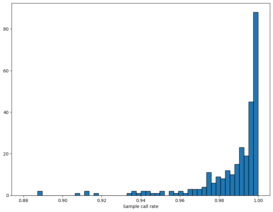
gq = ds.call_GQ.where(ds.call_GQ >= 0) # filter out missing
sample_gq_mean = gq.mean(dim="variants")
sample_gq_mean.attrs["long_name"] = "Mean Sample GQ"
xr.plot.hist(sample_gq_mean, range=(10,70), bins=60, size=8, edgecolor="black");
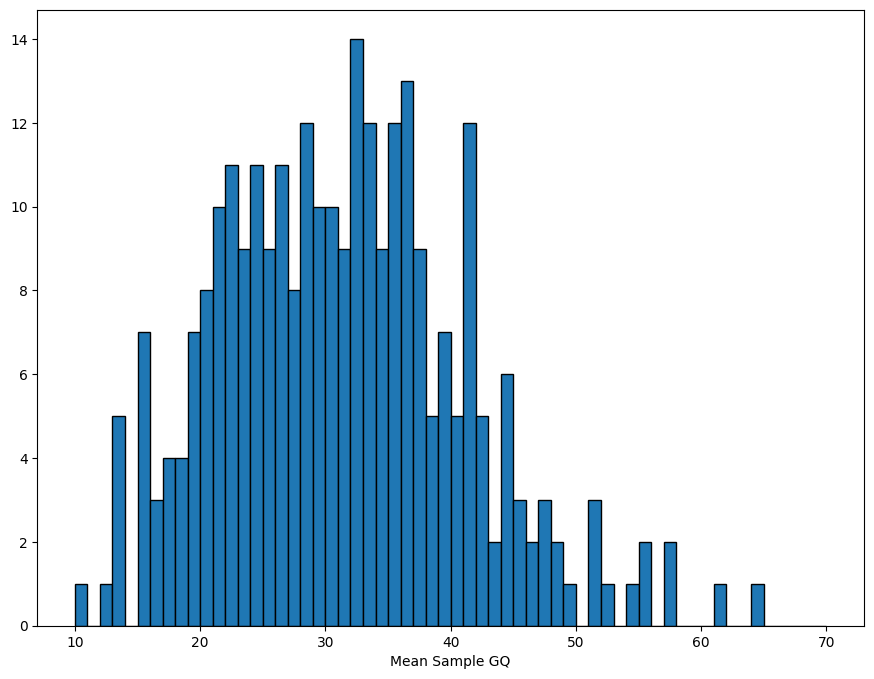
dp = ds.call_DP.where(ds.call_DP >= 0) # filter out missing
sample_dp_mean = dp.mean(dim="variants")
sample_dp_mean.attrs["long_name"] = "Mean Sample DP"
ds["sample_dp_mean"] = sample_dp_mean # add new data array to dataset
ds.plot.scatter(x="sample_dp_mean", y="sample_call_rate", size=8, s=10);
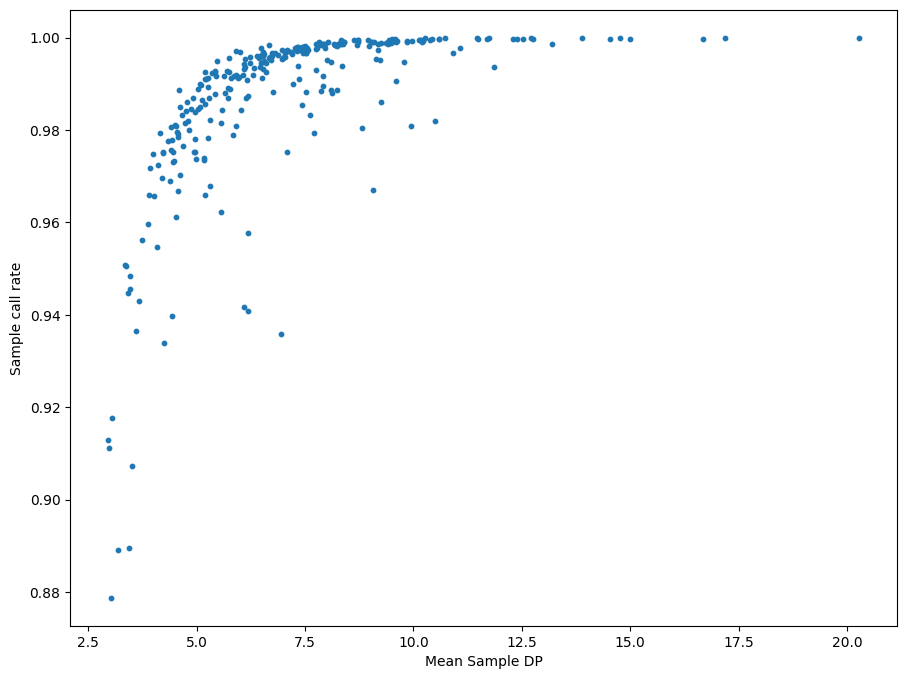
The following removes outliers using an arbitrary cutoff.
ds = ds.sel(samples=((ds.sample_dp_mean >= 4) & (ds.sample_call_rate >= 0.97)))
print(f"After filter, {len(ds.samples)}/284 samples remain.")
After filter, 250/284 samples remain.
Genotype QC is more complicated. First we calculate a variable ab, which is the fraction of reads that were the alternate allele.
# fill rows with nan where no alternate alleles were read or where sum of reads is 0
ad1 = ds.call_AD.sel(dict(alleles=1)).pipe(lambda v: v.where(v >= 0))
adsum = ds.call_AD.sum(dim="alleles").pipe(lambda v: v.where(v != 0))
# compute alternate allele read fraction
ab = ad1 / adsum
Then we can use the ab variable in the filter condition, to filter homozygous reference calls with >10% alternate reads, homozygous alternate calls with >10% reference reads, or heterozygote calls without a ref/alt balance near 50%.
GT = ds.call_genotype
hom_ref = (GT == 0).all(dim="ploidy")
het = GT[..., 0] != GT[..., 1]
hom_alt = ((GT > 0) & (GT[..., 0] == GT)).all(dim="ploidy")
filter_condition_ab = ((hom_ref & (ab <= 0.1)) |
                        (het & (ab >= 0.25) & (ab <= 0.75)) |
                        (hom_alt & (ab >= 0.9)))
filter_mask = xr.where(ds.call_genotype_mask, True, filter_condition_ab)
fraction_filtered = GT.where(~filter_mask).count().values / GT.size
print(f"Filtering {fraction_filtered * 100:.2f}% entries out of downstream analysis.")
Filtering 3.65% entries out of downstream analysis.
Note: genotype QC is filtering out slightly different numbers of entries compared to the Hail tutorial.
Variant QC is similar. This time we use the variant_stats function, but we won’t do any filtering on these variables.
ds = sg.variant_stats(ds)
ds
<xarray.Dataset>
Dimensions:                   (variants: 10879, alleles: 2, samples: 250,
                               ploidy: 2, contigs: 84, filters: 1)
Dimensions without coordinates: variants, alleles, samples, ploidy, contigs,
                                filters
Data variables: (12/38)
    variant_n_called          (variants) int64 dask.array<chunksize=(10000,), meta=np.ndarray>
    variant_call_rate         (variants) float64 dask.array<chunksize=(10000,), meta=np.ndarray>
    variant_n_het             (variants) int64 dask.array<chunksize=(10000,), meta=np.ndarray>
    variant_n_hom_ref         (variants) int64 dask.array<chunksize=(10000,), meta=np.ndarray>
    variant_n_hom_alt         (variants) int64 dask.array<chunksize=(10000,), meta=np.ndarray>
    variant_n_non_ref         (variants) int64 dask.array<chunksize=(10000,), meta=np.ndarray>
    ...                        ...
    Population                (samples) object 'GBR' 'GBR' 'GBR' ... 'GIH' 'GIH'
    SuperPopulation           (samples) object 'EUR' 'EUR' 'EUR' ... 'SAS' 'SAS'
    isFemale                  (samples) bool False True False ... False True
    PurpleHair                (samples) bool False False False ... True True
    CaffeineConsumption       (samples) int64 4 4 4 3 6 2 2 5 ... 6 4 6 4 6 5 5
    sample_dp_mean            (samples) float64 dask.array<chunksize=(250,), meta=np.ndarray>
Attributes: (7)- variants: 10879
- alleles: 2
- samples: 250
- ploidy: 2
- contigs: 84
- filters: 1
- variant_n_called(variants)int64dask.array<chunksize=(10000,), meta=np.ndarray>
- comment :
- The number of samples with called genotypes.
Array Chunk Bytes 84.99 kiB 78.12 kiB Shape (10879,) (10000,) Count 8 Graph Layers 2 Chunks Type int64 numpy.ndarray - variant_call_rate(variants)float64dask.array<chunksize=(10000,), meta=np.ndarray>
- comment :
- The fraction of samples with called genotypes.
Array Chunk Bytes 84.99 kiB 78.12 kiB Shape (10879,) (10000,) Count 9 Graph Layers 2 Chunks Type float64 numpy.ndarray - variant_n_het(variants)int64dask.array<chunksize=(10000,), meta=np.ndarray>
- comment :
- The number of samples with heterozygous calls.
Array Chunk Bytes 84.99 kiB 78.12 kiB Shape (10879,) (10000,) Count 24 Graph Layers 2 Chunks Type int64 numpy.ndarray - variant_n_hom_ref(variants)int64dask.array<chunksize=(10000,), meta=np.ndarray>
- comment :
- The number of samples with homozygous reference calls.
Array Chunk Bytes 84.99 kiB 78.12 kiB Shape (10879,) (10000,) Count 14 Graph Layers 2 Chunks Type int64 numpy.ndarray - variant_n_hom_alt(variants)int64dask.array<chunksize=(10000,), meta=np.ndarray>
- comment :
- The number of samples with homozygous alternate calls.
Array Chunk Bytes 84.99 kiB 78.12 kiB Shape (10879,) (10000,) Count 19 Graph Layers 2 Chunks Type int64 numpy.ndarray - variant_n_non_ref(variants)int64dask.array<chunksize=(10000,), meta=np.ndarray>
- comment :
- The number of samples that are not homozygous reference calls.
Array Chunk Bytes 84.99 kiB 78.12 kiB Shape (10879,) (10000,) Count 14 Graph Layers 2 Chunks Type int64 numpy.ndarray - variant_allele_count(variants, alleles)uint64dask.array<chunksize=(10000, 2), meta=np.ndarray>
- comment :
- Variant allele counts. With shape (variants, alleles) and values corresponding to the number of non-missing occurrences of each allele.
Array Chunk Bytes 169.98 kiB 156.25 kiB Shape (10879, 2) (10000, 2) Count 6 Graph Layers 2 Chunks Type uint64 numpy.ndarray - variant_allele_total(variants)int64dask.array<chunksize=(10000,), meta=np.ndarray>
- comment :
- The number of occurrences of all alleles.
Array Chunk Bytes 84.99 kiB 78.12 kiB Shape (10879,) (10000,) Count 7 Graph Layers 2 Chunks Type int64 numpy.ndarray - variant_allele_frequency(variants, alleles)float64dask.array<chunksize=(10000, 2), meta=np.ndarray>
- comment :
- The frequency of the occurrence of each allele.
Array Chunk Bytes 169.98 kiB 156.25 kiB Shape (10879, 2) (10000, 2) Count 16 Graph Layers 2 Chunks Type float64 numpy.ndarray - sample_n_called(samples)int64dask.array<chunksize=(250,), meta=np.ndarray>
- comment :
- The number of variants with called genotypes.
Array Chunk Bytes 1.95 kiB 1.95 kiB Shape (250,) (250,) Count 8 Graph Layers 1 Chunks Type int64 numpy.ndarray - sample_call_rate(samples)float64dask.array<chunksize=(250,), meta=np.ndarray>
- comment :
- The fraction of variants with called genotypes.
- long_name :
- Sample call rate
Array Chunk Bytes 1.95 kiB 1.95 kiB Shape (250,) (250,) Count 9 Graph Layers 1 Chunks Type float64 numpy.ndarray - sample_n_het(samples)int64dask.array<chunksize=(250,), meta=np.ndarray>
- comment :
- The number of variants with heterozygous calls.
Array Chunk Bytes 1.95 kiB 1.95 kiB Shape (250,) (250,) Count 23 Graph Layers 1 Chunks Type int64 numpy.ndarray - sample_n_hom_ref(samples)int64dask.array<chunksize=(250,), meta=np.ndarray>
- comment :
- The number of variants with homozygous reference calls.
Array Chunk Bytes 1.95 kiB 1.95 kiB Shape (250,) (250,) Count 13 Graph Layers 1 Chunks Type int64 numpy.ndarray - sample_n_hom_alt(samples)int64dask.array<chunksize=(250,), meta=np.ndarray>
- comment :
- The number of variants with homozygous alternate calls.
Array Chunk Bytes 1.95 kiB 1.95 kiB Shape (250,) (250,) Count 18 Graph Layers 1 Chunks Type int64 numpy.ndarray - sample_n_non_ref(samples)int64dask.array<chunksize=(250,), meta=np.ndarray>
- comment :
- The number of variants that are not homozygous reference calls.
Array Chunk Bytes 1.95 kiB 1.95 kiB Shape (250,) (250,) Count 13 Graph Layers 1 Chunks Type int64 numpy.ndarray - call_AD(variants, samples, alleles)int32dask.array<chunksize=(10000, 250, 2), meta=np.ndarray>
Array Chunk Bytes 20.75 MiB 19.07 MiB Shape (10879, 250, 2) (10000, 250, 2) Count 3 Graph Layers 2 Chunks Type int32 numpy.ndarray - call_DP(variants, samples)int32dask.array<chunksize=(10000, 250), meta=np.ndarray>
Array Chunk Bytes 10.38 MiB 9.54 MiB Shape (10879, 250) (10000, 250) Count 3 Graph Layers 2 Chunks Type int32 numpy.ndarray - call_GQ(variants, samples)int32dask.array<chunksize=(10000, 250), meta=np.ndarray>
Array Chunk Bytes 10.38 MiB 9.54 MiB Shape (10879, 250) (10000, 250) Count 3 Graph Layers 2 Chunks Type int32 numpy.ndarray - call_genotype(variants, samples, ploidy)int8dask.array<chunksize=(10000, 250, 2), meta=np.ndarray>
- comment :
- Call genotype. Encoded as allele values (0 for the reference, 1 for the first allele, 2 for the second allele), -1 to indicate a missing value, or -2 to indicate a non allele in mixed ploidy datasets.
- mixed_ploidy :
- False
Array Chunk Bytes 5.19 MiB 4.77 MiB Shape (10879, 250, 2) (10000, 250, 2) Count 3 Graph Layers 2 Chunks Type int8 numpy.ndarray - call_genotype_mask(variants, samples, ploidy)booldask.array<chunksize=(10000, 250, 2), meta=np.ndarray>
- comment :
- A flag for each call indicating which values are missing.
Array Chunk Bytes 5.19 MiB 4.77 MiB Shape (10879, 250, 2) (10000, 250, 2) Count 3 Graph Layers 2 Chunks Type bool numpy.ndarray - call_genotype_phased(variants, samples)booldask.array<chunksize=(10000, 250), meta=np.ndarray>
- comment :
- A flag for each call indicating if it is phased or not. If omitted all calls are unphased.
Array Chunk Bytes 2.59 MiB 2.38 MiB Shape (10879, 250) (10000, 250) Count 3 Graph Layers 2 Chunks Type bool numpy.ndarray - contig_id(contigs)<U10dask.array<chunksize=(84,), meta=np.ndarray>
- comment :
- Contig identifiers.
Array Chunk Bytes 3.28 kiB 3.28 kiB Shape (84,) (84,) Count 2 Graph Layers 1 Chunks Type numpy.ndarray - contig_length(contigs)int64dask.array<chunksize=(84,), meta=np.ndarray>
Array Chunk Bytes 672 B 672 B Shape (84,) (84,) Count 2 Graph Layers 1 Chunks Type int64 numpy.ndarray - filter_id(filters)objectdask.array<chunksize=(1,), meta=np.ndarray>
Array Chunk Bytes 8 B 8 B Shape (1,) (1,) Count 2 Graph Layers 1 Chunks Type object numpy.ndarray - variant_allele(variants, alleles)objectdask.array<chunksize=(10000, 2), meta=np.ndarray>
- comment :
- The possible alleles for the variant.
Array Chunk Bytes 169.98 kiB 156.25 kiB Shape (10879, 2) (10000, 2) Count 2 Graph Layers 2 Chunks Type object numpy.ndarray - variant_contig(variants)int8dask.array<chunksize=(10000,), meta=np.ndarray>
- comment :
- Index corresponding to contig name for each variant. In some less common scenarios, this may also be equivalent to the contig names if the data generating process used contig names that were also integers.
Array Chunk Bytes 10.62 kiB 9.77 kiB Shape (10879,) (10000,) Count 2 Graph Layers 2 Chunks Type int8 numpy.ndarray - variant_filter(variants, filters)booldask.array<chunksize=(10000, 1), meta=np.ndarray>
Array Chunk Bytes 10.62 kiB 9.77 kiB Shape (10879, 1) (10000, 1) Count 2 Graph Layers 2 Chunks Type bool numpy.ndarray - variant_id(variants)objectdask.array<chunksize=(10000,), meta=np.ndarray>
- comment :
- The unique identifier of the variant.
Array Chunk Bytes 84.99 kiB 78.12 kiB Shape (10879,) (10000,) Count 2 Graph Layers 2 Chunks Type object numpy.ndarray - variant_id_mask(variants)booldask.array<chunksize=(10000,), meta=np.ndarray>
Array Chunk Bytes 10.62 kiB 9.77 kiB Shape (10879,) (10000,) Count 2 Graph Layers 2 Chunks Type bool numpy.ndarray - variant_position(variants)int32dask.array<chunksize=(10000,), meta=np.ndarray>
- comment :
- The reference position of the variant.
Array Chunk Bytes 42.50 kiB 39.06 kiB Shape (10879,) (10000,) Count 2 Graph Layers 2 Chunks Type int32 numpy.ndarray - variant_quality(variants)float32dask.array<chunksize=(10000,), meta=np.ndarray>
Array Chunk Bytes 42.50 kiB 39.06 kiB Shape (10879,) (10000,) Count 2 Graph Layers 2 Chunks Type float32 numpy.ndarray - variant_contig_name(variants)int640 0 0 0 0 0 0 ... 22 22 22 22 22 22
array([ 0, 0, 0, ..., 22, 22, 22])
- Population(samples)object'GBR' 'GBR' 'GBR' ... 'GIH' 'GIH'
array(['GBR', 'GBR', 'GBR', 'GBR', 'GBR', 'GBR', 'GBR', 'FIN', 'FIN', 'FIN', 'CHS', 'CHS', 'CHS', 'CHS', 'CHS', 'CHS', 'CHS', 'CHS', 'CHS', 'CHS', 'CHS', 'CHS', 'PUR', 'CDX', 'PUR', 'PUR', 'PUR', 'PUR', 'PUR', 'PUR', 'PUR', 'CLM', 'CLM', 'CLM', 'GBR', 'CLM', 'PUR', 'CLM', 'CLM', 'CLM', 'IBS', 'PEL', 'IBS', 'IBS', 'IBS', 'IBS', 'IBS', 'GBR', 'CDX', 'CDX', 'CDX', 'CDX', 'CDX', 'CDX', 'KHV', 'KHV', 'KHV', 'KHV', 'KHV', 'ACB', 'PEL', 'PEL', 'PEL', 'PEL', 'ACB', 'KHV', 'ACB', 'KHV', 'KHV', 'KHV', 'KHV', 'KHV', 'CDX', 'CDX', 'CDX', 'IBS', 'IBS', 'CDX', 'PEL', 'PEL', 'PEL', 'CDX', 'CDX', 'CDX', 'CDX', 'CDX', 'CDX', 'CDX', 'CDX', 'CDX', 'ACB', 'GWD', 'GWD', 'ACB', 'KHV', 'GWD', 'GWD', 'ACB', 'GWD', 'PJL', 'GWD', 'PJL', 'PJL', 'PJL', 'PJL', 'PJL', 'GWD', 'GWD', 'GWD', 'PJL', 'GWD', 'GWD', 'GWD', 'GWD', 'GWD', 'GWD', 'ESN', 'ESN', 'BEB', 'GWD', 'MSL', 'MSL', 'ESN', 'ESN', 'ESN', 'MSL', 'PJL', 'GWD', 'GWD', 'GWD', 'ESN', 'ESN', 'ESN', 'ESN', 'MSL', 'MSL', 'MSL', 'MSL', 'PJL', 'PJL', 'ESN', 'MSL', 'MSL', 'BEB', 'BEB', 'BEB', 'PJL', 'STU', 'STU', 'STU', 'ITU', 'STU', 'STU', 'BEB', 'BEB', 'BEB', 'STU', 'ITU', 'STU', 'BEB', 'BEB', 'STU', 'ITU', 'ITU', 'ITU', 'ITU', 'STU', 'BEB', 'BEB', 'ITU', 'STU', 'STU', 'ITU', 'CEU', 'CEU', 'CEU', 'CEU', 'CEU', 'CEU', 'CEU', 'CEU', 'CEU', 'CEU', 'YRI', 'CHB', 'CHB', 'CHB', 'CHB', 'CHB', 'CHB', 'CHB', 'YRI', 'YRI', 'YRI', 'JPT', 'JPT', 'JPT', 'JPT', 'JPT', 'JPT', 'JPT', 'JPT', 'JPT', 'JPT', 'YRI', 'YRI', 'YRI', 'YRI', 'LWK', 'LWK', 'LWK', 'LWK', 'LWK', 'LWK', 'LWK', 'LWK', 'LWK', 'MXL', 'MXL', 'MXL', 'MXL', 'MXL', 'ASW', 'MXL', 'MXL', 'MXL', 'ASW', 'ASW', 'TSI', 'TSI', 'TSI', 'TSI', 'TSI', 'TSI', 'TSI', 'TSI', 'TSI', 'GIH', 'GIH', 'GIH', 'GIH', 'GIH', 'GIH', 'GIH', 'GIH', 'GIH', 'GIH', 'GIH', 'GIH', 'GIH'], dtype=object) - SuperPopulation(samples)object'EUR' 'EUR' 'EUR' ... 'SAS' 'SAS'
array(['EUR', 'EUR', 'EUR', 'EUR', 'EUR', 'EUR', 'EUR', 'EUR', 'EUR', 'EUR', 'EAS', 'EAS', 'EAS', 'EAS', 'EAS', 'EAS', 'EAS', 'EAS', 'EAS', 'EAS', 'EAS', 'EAS', 'AMR', 'EAS', 'AMR', 'AMR', 'AMR', 'AMR', 'AMR', 'AMR', 'AMR', 'AMR', 'AMR', 'AMR', 'EUR', 'AMR', 'AMR', 'AMR', 'AMR', 'AMR', 'EUR', 'AMR', 'EUR', 'EUR', 'EUR', 'EUR', 'EUR', 'EUR', 'EAS', 'EAS', 'EAS', 'EAS', 'EAS', 'EAS', 'EAS', 'EAS', 'EAS', 'EAS', 'EAS', 'AFR', 'AMR', 'AMR', 'AMR', 'AMR', 'AFR', 'EAS', 'AFR', 'EAS', 'EAS', 'EAS', 'EAS', 'EAS', 'EAS', 'EAS', 'EAS', 'EUR', 'EUR', 'EAS', 'AMR', 'AMR', 'AMR', 'EAS', 'EAS', 'EAS', 'EAS', 'EAS', 'EAS', 'EAS', 'EAS', 'EAS', 'AFR', 'AFR', 'AFR', 'AFR', 'EAS', 'AFR', 'AFR', 'AFR', 'AFR', 'SAS', 'AFR', 'SAS', 'SAS', 'SAS', 'SAS', 'SAS', 'AFR', 'AFR', 'AFR', 'SAS', 'AFR', 'AFR', 'AFR', 'AFR', 'AFR', 'AFR', 'AFR', 'AFR', 'SAS', 'AFR', 'AFR', 'AFR', 'AFR', 'AFR', 'AFR', 'AFR', 'SAS', 'AFR', 'AFR', 'AFR', 'AFR', 'AFR', 'AFR', 'AFR', 'AFR', 'AFR', 'AFR', 'AFR', 'SAS', 'SAS', 'AFR', 'AFR', 'AFR', 'SAS', 'SAS', 'SAS', 'SAS', 'SAS', 'SAS', 'SAS', 'SAS', 'SAS', 'SAS', 'SAS', 'SAS', 'SAS', 'SAS', 'SAS', 'SAS', 'SAS', 'SAS', 'SAS', 'SAS', 'SAS', 'SAS', 'SAS', 'SAS', 'SAS', 'SAS', 'SAS', 'SAS', 'SAS', 'SAS', 'EUR', 'EUR', 'EUR', 'EUR', 'EUR', 'EUR', 'EUR', 'EUR', 'EUR', 'EUR', 'AFR', 'EAS', 'EAS', 'EAS', 'EAS', 'EAS', 'EAS', 'EAS', 'AFR', 'AFR', 'AFR', 'EAS', 'EAS', 'EAS', 'EAS', 'EAS', 'EAS', 'EAS', 'EAS', 'EAS', 'EAS', 'AFR', 'AFR', 'AFR', 'AFR', 'AFR', 'AFR', 'AFR', 'AFR', 'AFR', 'AFR', 'AFR', 'AFR', 'AFR', 'AMR', 'AMR', 'AMR', 'AMR', 'AMR', 'AFR', 'AMR', 'AMR', 'AMR', 'AFR', 'AFR', 'EUR', 'EUR', 'EUR', 'EUR', 'EUR', 'EUR', 'EUR', 'EUR', 'EUR', 'SAS', 'SAS', 'SAS', 'SAS', 'SAS', 'SAS', 'SAS', 'SAS', 'SAS', 'SAS', 'SAS', 'SAS', 'SAS'], dtype=object) - isFemale(samples)boolFalse True False ... False True
array([False, True, False, True, False, False, True, False, True, False, False, True, False, True, False, False, False, True, True, True, False, True, True, False, True, True, False, False, True, False, True, False, True, True, False, True, True, False, False, True, True, True, False, True, False, False, True, True, True, True, True, True, True, True, True, False, True, True, True, True, True, True, False, False, True, False, True, True, True, False, False, True, True, True, True, True, False, False, False, True, True, False, False, False, False, False, False, False, False, False, True, True, False, True, False, False, True, True, True, False, True, False, True, True, False, False, True, False, False, False, False, True, True, True, True, False, True, False, False, True, False, True, True, False, False, False, False, True, True, True, True, True, True, False, True, True, False, True, False, True, True, False, True, True, False, True, False, True, False, True, True, False, False, False, False, True, False, True, True, False, True, True, True, True, True, False, True, False, True, True, False, False, False, False, True, False, False, True, False, True, False, False, True, False, True, False, True, True, False, True, False, False, True, True, False, False, True, True, True, False, False, False, False, True, False, False, True, True, True, False, True, False, True, False, True, True, True, False, True, False, True, False, True, False, False, True, False, False, True, False, True, True, True, False, True, False, True, False, False, True, True, True, True, True, False, False, False, False, False, True]) - PurpleHair(samples)boolFalse False False ... True True
array([False, False, False, False, False, True, False, False, True, True, False, False, True, True, True, True, True, True, True, False, True, True, False, False, False, False, False, True, False, True, True, True, False, True, False, True, False, False, False, False, True, False, False, True, False, False, True, True, False, True, False, False, False, False, False, True, True, False, False, True, True, True, False, False, True, False, True, True, True, True, True, True, True, True, False, True, True, True, True, True, False, False, False, True, False, True, True, False, False, False, False, True, False, True, False, True, True, True, True, True, True, True, False, True, False, False, False, True, True, False, False, True, True, True, True, True, False, False, True, True, False, False, False, False, False, True, False, False, False, False, True, False, False, False, False, False, False, False, False, True, False, False, True, True, True, False, True, False, True, True, True, True, True, True, False, False, False, False, False, False, True, True, True, True, False, False, True, False, True, True, False, False, True, False, False, True, True, True, True, True, True, False, True, True, False, False, True, True, True, False, True, False, False, False, True, True, True, False, False, False, False, False, True, False, False, False, True, False, False, True, False, False, False, False, False, True, False, True, True, False, False, False, False, True, False, True, False, True, True, False, False, False, False, True, True, True, True, True, True, False, False, True, False, False, True, True, True, False, True, True]) - CaffeineConsumption(samples)int644 4 4 3 6 2 2 5 ... 5 6 4 6 4 6 5 5
array([4, 4, 4, 3, 6, 2, 2, 5, 5, 4, 6, 5, 7, 5, 7, 1, 5, 5, 4, 4, 5, 5, 5, 6, 4, 4, 6, 3, 3, 5, 4, 4, 5, 5, 4, 6, 5, 4, 4, 5, 6, 3, 7, 5, 5, 6, 3, 2, 5, 5, 4, 6, 5, 6, 4, 6, 7, 6, 7, 3, 5, 6, 5, 6, 4, 5, 4, 4, 5, 8, 3, 4, 4, 7, 5, 2, 6, 7, 6, 5, 3, 4, 5, 5, 5, 5, 6, 4, 5, 7, 2, 3, 3, 2, 6, 4, 2, 6, 5, 3, 4, 7, 6, 7, 6, 3, 4, 2, 2, 5, 6, 7, 8, 6, 2, 3, 2, 0, 5, 7, 5, 1, 4, 3, 2, 4, 6, 5, 4, 4, 1, 5, 5, 3, 1, 1, 3, 2, 4, 2, 1, 3, 3, 4, 4, 5, 6, 5, 4, 5, 0, 4, 5, 4, 3, 3, 4, 4, 3, 5, 6, 5, 3, 4, 4, 6, 3, 5, 5, 4, 5, 3, 5, 4, 6, 5, 7, 5, 6, 6, 4, 4, 5, 3, 5, 4, 3, 8, 4, 6, 8, 3, 4, 2, 5, 6, 6, 4, 3, 5, 7, 4, 5, 5, 6, 3, 2, 4, 5, 6, 7, 2, 4, 2, 1, 5, 3, 4, 9, 6, 4, 3, 4, 4, 6, 7, 6, 3, 4, 3, 6, 6, 3, 4, 4, 4, 6, 7, 4, 5, 4, 5, 5, 6, 4, 6, 4, 6, 5, 5]) - sample_dp_mean(samples)float64dask.array<chunksize=(250,), meta=np.ndarray>
- long_name :
- Mean Sample DP
Array Chunk Bytes 1.95 kiB 1.95 kiB Shape (250,) (250,) Count 8 Graph Layers 1 Chunks Type float64 numpy.ndarray
- contig_lengths :
- [249250621, 243199373, 198022430, 191154276, 180915260, 171115067, 159138663, 146364022, 141213431, 135534747, 135006516, 133851895, 115169878, 107349540, 102531392, 90354753, 81195210, 78077248, 59128983, 63025520, 48129895, 51304566, 155270560, 59373566, 16569, 4262, 15008, 19913, 27386, 27682, 33824, 34474, 36148, 36422, 36651, 37175, 37498, 38154, 38502, 38914, 39786, 39929, 39939, 40103, 40531, 40652, 41001, 41933, 41934, 42152, 43341, 43523, 43691, 45867, 45941, 81310, 90085, 92689, 106433, 128374, 129120, 137718, 155397, 159169, 161147, 161802, 164239, 166566, 169874, 172149, 172294, 172545, 174588, 179198, 179693, 180455, 182896, 186858, 186861, 187035, 189789, 191469, 211173, 547496]
- contigs :
- ['1', '2', '3', '4', '5', '6', '7', '8', '9', '10', '11', '12', '13', '14', '15', '16', '17', '18', '19', '20', '21', '22', 'X', 'Y', 'MT', 'GL000207.1', 'GL000226.1', 'GL000229.1', 'GL000231.1', 'GL000210.1', 'GL000239.1', 'GL000235.1', 'GL000201.1', 'GL000247.1', 'GL000245.1', 'GL000197.1', 'GL000203.1', 'GL000246.1', 'GL000249.1', 'GL000196.1', 'GL000248.1', 'GL000244.1', 'GL000238.1', 'GL000202.1', 'GL000234.1', 'GL000232.1', 'GL000206.1', 'GL000240.1', 'GL000236.1', 'GL000241.1', 'GL000243.1', 'GL000242.1', 'GL000230.1', 'GL000237.1', 'GL000233.1', 'GL000204.1', 'GL000198.1', 'GL000208.1', 'GL000191.1', 'GL000227.1', 'GL000228.1', 'GL000214.1', 'GL000221.1', 'GL000209.1', 'GL000218.1', 'GL000220.1', 'GL000213.1', 'GL000211.1', 'GL000199.1', 'GL000217.1', 'GL000216.1', 'GL000215.1', 'GL000205.1', 'GL000219.1', 'GL000224.1', 'GL000223.1', 'GL000195.1', 'GL000212.1', 'GL000222.1', 'GL000200.1', 'GL000193.1', 'GL000194.1', 'GL000225.1', 'GL000192.1']
- filters :
- ['PASS']
- max_alt_alleles_seen :
- 1
- source :
- sgkit-0.6.1.dev2+gcc728043
- vcf_header :
- ##fileformat=VCFv4.2 ##FILTER=<ID=PASS,Description="All filters passed"> ##hailversion=0.2-29fbaeaf265e ##FORMAT=<ID=GT,Number=1,Type=String,Description=""> ##FORMAT=<ID=AD,Number=.,Type=Integer,Description=""> ##FORMAT=<ID=DP,Number=1,Type=Integer,Description=""> ##FORMAT=<ID=GQ,Number=1,Type=Integer,Description=""> ##FORMAT=<ID=PL,Number=.,Type=Integer,Description=""> ##INFO=<ID=AC,Number=.,Type=Integer,Description=""> ##INFO=<ID=AF,Number=.,Type=Float,Description=""> ##INFO=<ID=AN,Number=1,Type=Integer,Description=""> ##INFO=<ID=BaseQRankSum,Number=1,Type=Float,Description=""> ##INFO=<ID=ClippingRankSum,Number=1,Type=Float,Description=""> ##INFO=<ID=DP,Number=1,Type=Integer,Description=""> ##INFO=<ID=DS,Number=0,Type=Flag,Description=""> ##INFO=<ID=FS,Number=1,Type=Float,Description=""> ##INFO=<ID=HaplotypeScore,Number=1,Type=Float,Description=""> ##INFO=<ID=InbreedingCoeff,Number=1,Type=Float,Description=""> ##INFO=<ID=MLEAC,Number=.,Type=Integer,Description=""> ##INFO=<ID=MLEAF,Number=.,Type=Float,Description=""> ##INFO=<ID=MQ,Number=1,Type=Float,Description=""> ##INFO=<ID=MQ0,Number=1,Type=Integer,Description=""> ##INFO=<ID=MQRankSum,Number=1,Type=Float,Description=""> ##INFO=<ID=QD,Number=1,Type=Float,Description=""> ##INFO=<ID=ReadPosRankSum,Number=1,Type=Float,Description=""> ##INFO=<ID=set,Number=1,Type=String,Description=""> ##contig=<ID=1,length=249250621,assembly=GRCh37> ##contig=<ID=2,length=243199373,assembly=GRCh37> ##contig=<ID=3,length=198022430,assembly=GRCh37> ##contig=<ID=4,length=191154276,assembly=GRCh37> ##contig=<ID=5,length=180915260,assembly=GRCh37> ##contig=<ID=6,length=171115067,assembly=GRCh37> ##contig=<ID=7,length=159138663,assembly=GRCh37> ##contig=<ID=8,length=146364022,assembly=GRCh37> ##contig=<ID=9,length=141213431,assembly=GRCh37> ##contig=<ID=10,length=135534747,assembly=GRCh37> ##contig=<ID=11,length=135006516,assembly=GRCh37> ##contig=<ID=12,length=133851895,assembly=GRCh37> ##contig=<ID=13,length=115169878,assembly=GRCh37> ##contig=<ID=14,length=107349540,assembly=GRCh37> ##contig=<ID=15,length=102531392,assembly=GRCh37> ##contig=<ID=16,length=90354753,assembly=GRCh37> ##contig=<ID=17,length=81195210,assembly=GRCh37> ##contig=<ID=18,length=78077248,assembly=GRCh37> ##contig=<ID=19,length=59128983,assembly=GRCh37> ##contig=<ID=20,length=63025520,assembly=GRCh37> ##contig=<ID=21,length=48129895,assembly=GRCh37> ##contig=<ID=22,length=51304566,assembly=GRCh37> ##contig=<ID=X,length=155270560,assembly=GRCh37> ##contig=<ID=Y,length=59373566,assembly=GRCh37> ##contig=<ID=MT,length=16569,assembly=GRCh37> ##contig=<ID=GL000207.1,length=4262,assembly=GRCh37> ##contig=<ID=GL000226.1,length=15008,assembly=GRCh37> ##contig=<ID=GL000229.1,length=19913,assembly=GRCh37> ##contig=<ID=GL000231.1,length=27386,assembly=GRCh37> ##contig=<ID=GL000210.1,length=27682,assembly=GRCh37> ##contig=<ID=GL000239.1,length=33824,assembly=GRCh37> ##contig=<ID=GL000235.1,length=34474,assembly=GRCh37> ##contig=<ID=GL000201.1,length=36148,assembly=GRCh37> ##contig=<ID=GL000247.1,length=36422,assembly=GRCh37> ##contig=<ID=GL000245.1,length=36651,assembly=GRCh37> ##contig=<ID=GL000197.1,length=37175,assembly=GRCh37> ##contig=<ID=GL000203.1,length=37498,assembly=GRCh37> ##contig=<ID=GL000246.1,length=38154,assembly=GRCh37> ##contig=<ID=GL000249.1,length=38502,assembly=GRCh37> ##contig=<ID=GL000196.1,length=38914,assembly=GRCh37> ##contig=<ID=GL000248.1,length=39786,assembly=GRCh37> ##contig=<ID=GL000244.1,length=39929,assembly=GRCh37> ##contig=<ID=GL000238.1,length=39939,assembly=GRCh37> ##contig=<ID=GL000202.1,length=40103,assembly=GRCh37> ##contig=<ID=GL000234.1,length=40531,assembly=GRCh37> ##contig=<ID=GL000232.1,length=40652,assembly=GRCh37> ##contig=<ID=GL000206.1,length=41001,assembly=GRCh37> ##contig=<ID=GL000240.1,length=41933,assembly=GRCh37> ##contig=<ID=GL000236.1,length=41934,assembly=GRCh37> ##contig=<ID=GL000241.1,length=42152,assembly=GRCh37> ##contig=<ID=GL000243.1,length=43341,assembly=GRCh37> ##contig=<ID=GL000242.1,length=43523,assembly=GRCh37> ##contig=<ID=GL000230.1,length=43691,assembly=GRCh37> ##contig=<ID=GL000237.1,length=45867,assembly=GRCh37> ##contig=<ID=GL000233.1,length=45941,assembly=GRCh37> ##contig=<ID=GL000204.1,length=81310,assembly=GRCh37> ##contig=<ID=GL000198.1,length=90085,assembly=GRCh37> ##contig=<ID=GL000208.1,length=92689,assembly=GRCh37> ##contig=<ID=GL000191.1,length=106433,assembly=GRCh37> ##contig=<ID=GL000227.1,length=128374,assembly=GRCh37> ##contig=<ID=GL000228.1,length=129120,assembly=GRCh37> ##contig=<ID=GL000214.1,length=137718,assembly=GRCh37> ##contig=<ID=GL000221.1,length=155397,assembly=GRCh37> ##contig=<ID=GL000209.1,length=159169,assembly=GRCh37> ##contig=<ID=GL000218.1,length=161147,assembly=GRCh37> ##contig=<ID=GL000220.1,length=161802,assembly=GRCh37> ##contig=<ID=GL000213.1,length=164239,assembly=GRCh37> ##contig=<ID=GL000211.1,length=166566,assembly=GRCh37> ##contig=<ID=GL000199.1,length=169874,assembly=GRCh37> ##contig=<ID=GL000217.1,length=172149,assembly=GRCh37> ##contig=<ID=GL000216.1,length=172294,assembly=GRCh37> ##contig=<ID=GL000215.1,length=172545,assembly=GRCh37> ##contig=<ID=GL000205.1,length=174588,assembly=GRCh37> ##contig=<ID=GL000219.1,length=179198,assembly=GRCh37> ##contig=<ID=GL000224.1,length=179693,assembly=GRCh37> ##contig=<ID=GL000223.1,length=180455,assembly=GRCh37> ##contig=<ID=GL000195.1,length=182896,assembly=GRCh37> ##contig=<ID=GL000212.1,length=186858,assembly=GRCh37> ##contig=<ID=GL000222.1,length=186861,assembly=GRCh37> ##contig=<ID=GL000200.1,length=187035,assembly=GRCh37> ##contig=<ID=GL000193.1,length=189789,assembly=GRCh37> ##contig=<ID=GL000194.1,length=191469,assembly=GRCh37> ##contig=<ID=GL000225.1,length=211173,assembly=GRCh37> ##contig=<ID=GL000192.1,length=547496,assembly=GRCh37> #CHROM POS ID REF ALT QUAL FILTER INFO FORMAT HG00096 HG00099 HG00105 HG00118 HG00129 HG00148 HG00177 HG00182 HG00242 HG00254 HG00265 HG00271 HG00274 HG00332 HG00335 HG00369 HG00421 HG00436 HG00452 HG00472 HG00530 HG00534 HG00583 HG00590 HG00598 HG00607 HG00619 HG00623 HG00657 HG00663 HG00704 HG00705 HG00733 HG00864 HG00881 HG01052 HG01070 HG01075 HG01164 HG01174 HG01241 HG01248 HG01256 HG01275 HG01284 HG01334 HG01348 HG01396 HG01443 HG01491 HG01498 HG01537 HG01572 HG01606 HG01623 HG01630 HG01783 HG01784 HG01790 HG01799 HG01801 HG01806 HG01812 HG01813 HG01817 HG01848 HG01849 HG01857 HG01863 HG01874 HG01915 HG01924 HG01965 HG01970 HG01991 HG02010 HG02020 HG02054 HG02086 HG02087 HG02116 HG02122 HG02130 HG02131 HG02152 HG02154 HG02165 HG02224 HG02232 HG02236 HG02250 HG02259 HG02298 HG02318 HG02345 HG02351 HG02363 HG02373 HG02383 HG02384 HG02386 HG02388 HG02389 HG02397 HG02419 HG02462 HG02464 HG02497 HG02511 HG02521 HG02561 HG02574 HG02580 HG02595 HG02603 HG02629 HG02651 HG02682 HG02688 HG02690 HG02699 HG02760 HG02768 HG02771 HG02792 HG02798 HG02811 HG02814 HG02840 HG02870 HG02881 HG02970 HG02973 HG03009 HG03046 HG03074 HG03091 HG03105 HG03127 HG03193 HG03224 HG03237 HG03241 HG03247 HG03259 HG03267 HG03354 HG03366 HG03367 HG03380 HG03419 HG03449 HG03451 HG03458 HG03490 HG03491 HG03511 HG03556 HG03563 HG03598 HG03603 HG03607 HG03636 HG03684 HG03686 HG03690 HG03731 HG03740 HG03755 HG03800 HG03815 HG03832 HG03850 HG03873 HG03897 HG03905 HG03937 HG03948 HG03973 HG04054 HG04059 HG04063 HG04096 HG04099 HG04140 HG04171 HG04209 HG04210 HG04229 HG04239 NA07347 NA11918 NA11919 NA12045 NA12273 NA12342 NA12414 NA12546 NA12760 NA12878 NA18516 NA18525 NA18534 NA18541 NA18557 NA18565 NA18616 NA18619 NA18623 NA18630 NA18631 NA18740 NA18853 NA18865 NA18873 NA18874 NA18916 NA18960 NA18966 NA18975 NA18976 NA18978 NA18990 NA19060 NA19063 NA19076 NA19086 NA19087 NA19096 NA19113 NA19118 NA19185 NA19209 NA19311 NA19314 NA19317 NA19321 NA19379 NA19384 NA19390 NA19397 NA19399 NA19404 NA19446 NA19448 NA19455 NA19456 NA19466 NA19655 NA19657 NA19670 NA19678 NA19679 NA19701 NA19720 NA19756 NA19761 NA19764 NA19786 NA20318 NA20351 NA20517 NA20518 NA20529 NA20587 NA20757 NA20798 NA20799 NA20800 NA20810 NA20826 NA20858 NA20864 NA20869 NA20877 NA20888 NA20910 NA21101 NA21113 NA21114 NA21116 NA21118 NA21133 NA21143
- vcf_zarr_version :
- 0.2
Let’s do a GWAS!#
First we need to restrict to common variants (1% cutoff), and not far from Hardy-Weinberg equilibrium.
ds = sg.hardy_weinberg_test(ds)
(The warning is telling us that some variables are being regenerated, and can be safely ignored.)
ds
<xarray.Dataset>
Dimensions:                   (variants: 10879, genotypes: 3, alleles: 2,
                               samples: 250, ploidy: 2, contigs: 84, filters: 1)
Coordinates:
  * genotypes                 (genotypes) <U3 '0/0' '0/1' '1/1'
Dimensions without coordinates: variants, alleles, samples, ploidy, contigs,
                                filters
Data variables: (12/41)
    variant_hwe_p_value       (variants) float64 dask.array<chunksize=(10000,), meta=np.ndarray>
    variant_genotype_count    (variants, genotypes) uint64 dask.array<chunksize=(10000, 3), meta=np.ndarray>
    genotype_id               (genotypes) <U3 dask.array<chunksize=(3,), meta=np.ndarray>
    variant_n_called          (variants) int64 dask.array<chunksize=(10000,), meta=np.ndarray>
    variant_call_rate         (variants) float64 dask.array<chunksize=(10000,), meta=np.ndarray>
    variant_n_het             (variants) int64 dask.array<chunksize=(10000,), meta=np.ndarray>
    ...                        ...
    Population                (samples) object 'GBR' 'GBR' 'GBR' ... 'GIH' 'GIH'
    SuperPopulation           (samples) object 'EUR' 'EUR' 'EUR' ... 'SAS' 'SAS'
    isFemale                  (samples) bool False True False ... False True
    PurpleHair                (samples) bool False False False ... True True
    CaffeineConsumption       (samples) int64 4 4 4 3 6 2 2 5 ... 6 4 6 4 6 5 5
    sample_dp_mean            (samples) float64 dask.array<chunksize=(250,), meta=np.ndarray>
Attributes: (7)- variants: 10879
- genotypes: 3
- alleles: 2
- samples: 250
- ploidy: 2
- contigs: 84
- filters: 1
- genotypes(genotypes)<U3'0/0' '0/1' '1/1'
array(['0/0', '0/1', '1/1'], dtype='<U3')
- variant_hwe_p_value(variants)float64dask.array<chunksize=(10000,), meta=np.ndarray>
- comment :
- P values from HWE test for each variant as float in [0, 1].
Array Chunk Bytes 84.99 kiB 78.12 kiB Shape (10879,) (10000,) Count 8 Graph Layers 2 Chunks Type float64 numpy.ndarray - variant_genotype_count(variants, genotypes)uint64dask.array<chunksize=(10000, 3), meta=np.ndarray>
- comment :
- The number of observations for each possible genotype at each variant. Counts are sorted following the ordering defined in the VCF specification. - For biallelic, diploid genotypes the ordering is ``00``, ``01``, ``11`` (homozygous reference, heterozygous, homozygous alternate). - For triallelic, diploid genotypes the ordering is ``00``, ``01``, ``11``, ``02``, ``12``, ``22`` - For triallelic, triploid genotypes the ordering is ``000``, ``001``, ``011``, ``111``, ``002``, ``012``, ``112``, ``022``, ``122``, ``222``
Array Chunk Bytes 254.98 kiB 234.38 kiB Shape (10879, 3) (10000, 3) Count 4 Graph Layers 2 Chunks Type uint64 numpy.ndarray - genotype_id(genotypes)<U3dask.array<chunksize=(3,), meta=np.ndarray>
- comment :
- VCF style genotype strings for all possible genotypes given the size of the ploidy and alleles dimensions. The ordering of genotype strings follows the ordering outlined in the VCF specification for arrays of size "G".
Array Chunk Bytes 36 B 36 B Shape (3,) (3,) Count 4 Graph Layers 1 Chunks Type numpy.ndarray - variant_n_called(variants)int64dask.array<chunksize=(10000,), meta=np.ndarray>
- comment :
- The number of samples with called genotypes.
Array Chunk Bytes 84.99 kiB 78.12 kiB Shape (10879,) (10000,) Count 8 Graph Layers 2 Chunks Type int64 numpy.ndarray - variant_call_rate(variants)float64dask.array<chunksize=(10000,), meta=np.ndarray>
- comment :
- The fraction of samples with called genotypes.
Array Chunk Bytes 84.99 kiB 78.12 kiB Shape (10879,) (10000,) Count 9 Graph Layers 2 Chunks Type float64 numpy.ndarray - variant_n_het(variants)int64dask.array<chunksize=(10000,), meta=np.ndarray>
- comment :
- The number of samples with heterozygous calls.
Array Chunk Bytes 84.99 kiB 78.12 kiB Shape (10879,) (10000,) Count 24 Graph Layers 2 Chunks Type int64 numpy.ndarray - variant_n_hom_ref(variants)int64dask.array<chunksize=(10000,), meta=np.ndarray>
- comment :
- The number of samples with homozygous reference calls.
Array Chunk Bytes 84.99 kiB 78.12 kiB Shape (10879,) (10000,) Count 14 Graph Layers 2 Chunks Type int64 numpy.ndarray - variant_n_hom_alt(variants)int64dask.array<chunksize=(10000,), meta=np.ndarray>
- comment :
- The number of samples with homozygous alternate calls.
Array Chunk Bytes 84.99 kiB 78.12 kiB Shape (10879,) (10000,) Count 19 Graph Layers 2 Chunks Type int64 numpy.ndarray - variant_n_non_ref(variants)int64dask.array<chunksize=(10000,), meta=np.ndarray>
- comment :
- The number of samples that are not homozygous reference calls.
Array Chunk Bytes 84.99 kiB 78.12 kiB Shape (10879,) (10000,) Count 14 Graph Layers 2 Chunks Type int64 numpy.ndarray - variant_allele_count(variants, alleles)uint64dask.array<chunksize=(10000, 2), meta=np.ndarray>
- comment :
- Variant allele counts. With shape (variants, alleles) and values corresponding to the number of non-missing occurrences of each allele.
Array Chunk Bytes 169.98 kiB 156.25 kiB Shape (10879, 2) (10000, 2) Count 6 Graph Layers 2 Chunks Type uint64 numpy.ndarray - variant_allele_total(variants)int64dask.array<chunksize=(10000,), meta=np.ndarray>
- comment :
- The number of occurrences of all alleles.
Array Chunk Bytes 84.99 kiB 78.12 kiB Shape (10879,) (10000,) Count 7 Graph Layers 2 Chunks Type int64 numpy.ndarray - variant_allele_frequency(variants, alleles)float64dask.array<chunksize=(10000, 2), meta=np.ndarray>
- comment :
- The frequency of the occurrence of each allele.
Array Chunk Bytes 169.98 kiB 156.25 kiB Shape (10879, 2) (10000, 2) Count 16 Graph Layers 2 Chunks Type float64 numpy.ndarray - sample_n_called(samples)int64dask.array<chunksize=(250,), meta=np.ndarray>
- comment :
- The number of variants with called genotypes.
Array Chunk Bytes 1.95 kiB 1.95 kiB Shape (250,) (250,) Count 8 Graph Layers 1 Chunks Type int64 numpy.ndarray - sample_call_rate(samples)float64dask.array<chunksize=(250,), meta=np.ndarray>
- comment :
- The fraction of variants with called genotypes.
- long_name :
- Sample call rate
Array Chunk Bytes 1.95 kiB 1.95 kiB Shape (250,) (250,) Count 9 Graph Layers 1 Chunks Type float64 numpy.ndarray - sample_n_het(samples)int64dask.array<chunksize=(250,), meta=np.ndarray>
- comment :
- The number of variants with heterozygous calls.
Array Chunk Bytes 1.95 kiB 1.95 kiB Shape (250,) (250,) Count 23 Graph Layers 1 Chunks Type int64 numpy.ndarray - sample_n_hom_ref(samples)int64dask.array<chunksize=(250,), meta=np.ndarray>
- comment :
- The number of variants with homozygous reference calls.
Array Chunk Bytes 1.95 kiB 1.95 kiB Shape (250,) (250,) Count 13 Graph Layers 1 Chunks Type int64 numpy.ndarray - sample_n_hom_alt(samples)int64dask.array<chunksize=(250,), meta=np.ndarray>
- comment :
- The number of variants with homozygous alternate calls.
Array Chunk Bytes 1.95 kiB 1.95 kiB Shape (250,) (250,) Count 18 Graph Layers 1 Chunks Type int64 numpy.ndarray - sample_n_non_ref(samples)int64dask.array<chunksize=(250,), meta=np.ndarray>
- comment :
- The number of variants that are not homozygous reference calls.
Array Chunk Bytes 1.95 kiB 1.95 kiB Shape (250,) (250,) Count 13 Graph Layers 1 Chunks Type int64 numpy.ndarray - call_AD(variants, samples, alleles)int32dask.array<chunksize=(10000, 250, 2), meta=np.ndarray>
Array Chunk Bytes 20.75 MiB 19.07 MiB Shape (10879, 250, 2) (10000, 250, 2) Count 3 Graph Layers 2 Chunks Type int32 numpy.ndarray - call_DP(variants, samples)int32dask.array<chunksize=(10000, 250), meta=np.ndarray>
Array Chunk Bytes 10.38 MiB 9.54 MiB Shape (10879, 250) (10000, 250) Count 3 Graph Layers 2 Chunks Type int32 numpy.ndarray - call_GQ(variants, samples)int32dask.array<chunksize=(10000, 250), meta=np.ndarray>
Array Chunk Bytes 10.38 MiB 9.54 MiB Shape (10879, 250) (10000, 250) Count 3 Graph Layers 2 Chunks Type int32 numpy.ndarray - call_genotype(variants, samples, ploidy)int8dask.array<chunksize=(10000, 250, 2), meta=np.ndarray>
- comment :
- Call genotype. Encoded as allele values (0 for the reference, 1 for the first allele, 2 for the second allele), -1 to indicate a missing value, or -2 to indicate a non allele in mixed ploidy datasets.
- mixed_ploidy :
- False
Array Chunk Bytes 5.19 MiB 4.77 MiB Shape (10879, 250, 2) (10000, 250, 2) Count 3 Graph Layers 2 Chunks Type int8 numpy.ndarray - call_genotype_mask(variants, samples, ploidy)booldask.array<chunksize=(10000, 250, 2), meta=np.ndarray>
- comment :
- A flag for each call indicating which values are missing.
Array Chunk Bytes 5.19 MiB 4.77 MiB Shape (10879, 250, 2) (10000, 250, 2) Count 3 Graph Layers 2 Chunks Type bool numpy.ndarray - call_genotype_phased(variants, samples)booldask.array<chunksize=(10000, 250), meta=np.ndarray>
- comment :
- A flag for each call indicating if it is phased or not. If omitted all calls are unphased.
Array Chunk Bytes 2.59 MiB 2.38 MiB Shape (10879, 250) (10000, 250) Count 3 Graph Layers 2 Chunks Type bool numpy.ndarray - contig_id(contigs)<U10dask.array<chunksize=(84,), meta=np.ndarray>
- comment :
- Contig identifiers.
Array Chunk Bytes 3.28 kiB 3.28 kiB Shape (84,) (84,) Count 2 Graph Layers 1 Chunks Type numpy.ndarray - contig_length(contigs)int64dask.array<chunksize=(84,), meta=np.ndarray>
Array Chunk Bytes 672 B 672 B Shape (84,) (84,) Count 2 Graph Layers 1 Chunks Type int64 numpy.ndarray - filter_id(filters)objectdask.array<chunksize=(1,), meta=np.ndarray>
Array Chunk Bytes 8 B 8 B Shape (1,) (1,) Count 2 Graph Layers 1 Chunks Type object numpy.ndarray - variant_allele(variants, alleles)objectdask.array<chunksize=(10000, 2), meta=np.ndarray>
- comment :
- The possible alleles for the variant.
Array Chunk Bytes 169.98 kiB 156.25 kiB Shape (10879, 2) (10000, 2) Count 2 Graph Layers 2 Chunks Type object numpy.ndarray - variant_contig(variants)int8dask.array<chunksize=(10000,), meta=np.ndarray>
- comment :
- Index corresponding to contig name for each variant. In some less common scenarios, this may also be equivalent to the contig names if the data generating process used contig names that were also integers.
Array Chunk Bytes 10.62 kiB 9.77 kiB Shape (10879,) (10000,) Count 2 Graph Layers 2 Chunks Type int8 numpy.ndarray - variant_filter(variants, filters)booldask.array<chunksize=(10000, 1), meta=np.ndarray>
Array Chunk Bytes 10.62 kiB 9.77 kiB Shape (10879, 1) (10000, 1) Count 2 Graph Layers 2 Chunks Type bool numpy.ndarray - variant_id(variants)objectdask.array<chunksize=(10000,), meta=np.ndarray>
- comment :
- The unique identifier of the variant.
Array Chunk Bytes 84.99 kiB 78.12 kiB Shape (10879,) (10000,) Count 2 Graph Layers 2 Chunks Type object numpy.ndarray - variant_id_mask(variants)booldask.array<chunksize=(10000,), meta=np.ndarray>
Array Chunk Bytes 10.62 kiB 9.77 kiB Shape (10879,) (10000,) Count 2 Graph Layers 2 Chunks Type bool numpy.ndarray - variant_position(variants)int32dask.array<chunksize=(10000,), meta=np.ndarray>
- comment :
- The reference position of the variant.
Array Chunk Bytes 42.50 kiB 39.06 kiB Shape (10879,) (10000,) Count 2 Graph Layers 2 Chunks Type int32 numpy.ndarray - variant_quality(variants)float32dask.array<chunksize=(10000,), meta=np.ndarray>
Array Chunk Bytes 42.50 kiB 39.06 kiB Shape (10879,) (10000,) Count 2 Graph Layers 2 Chunks Type float32 numpy.ndarray - variant_contig_name(variants)int640 0 0 0 0 0 0 ... 22 22 22 22 22 22
array([ 0, 0, 0, ..., 22, 22, 22])
- Population(samples)object'GBR' 'GBR' 'GBR' ... 'GIH' 'GIH'
array(['GBR', 'GBR', 'GBR', 'GBR', 'GBR', 'GBR', 'GBR', 'FIN', 'FIN', 'FIN', 'CHS', 'CHS', 'CHS', 'CHS', 'CHS', 'CHS', 'CHS', 'CHS', 'CHS', 'CHS', 'CHS', 'CHS', 'PUR', 'CDX', 'PUR', 'PUR', 'PUR', 'PUR', 'PUR', 'PUR', 'PUR', 'CLM', 'CLM', 'CLM', 'GBR', 'CLM', 'PUR', 'CLM', 'CLM', 'CLM', 'IBS', 'PEL', 'IBS', 'IBS', 'IBS', 'IBS', 'IBS', 'GBR', 'CDX', 'CDX', 'CDX', 'CDX', 'CDX', 'CDX', 'KHV', 'KHV', 'KHV', 'KHV', 'KHV', 'ACB', 'PEL', 'PEL', 'PEL', 'PEL', 'ACB', 'KHV', 'ACB', 'KHV', 'KHV', 'KHV', 'KHV', 'KHV', 'CDX', 'CDX', 'CDX', 'IBS', 'IBS', 'CDX', 'PEL', 'PEL', 'PEL', 'CDX', 'CDX', 'CDX', 'CDX', 'CDX', 'CDX', 'CDX', 'CDX', 'CDX', 'ACB', 'GWD', 'GWD', 'ACB', 'KHV', 'GWD', 'GWD', 'ACB', 'GWD', 'PJL', 'GWD', 'PJL', 'PJL', 'PJL', 'PJL', 'PJL', 'GWD', 'GWD', 'GWD', 'PJL', 'GWD', 'GWD', 'GWD', 'GWD', 'GWD', 'GWD', 'ESN', 'ESN', 'BEB', 'GWD', 'MSL', 'MSL', 'ESN', 'ESN', 'ESN', 'MSL', 'PJL', 'GWD', 'GWD', 'GWD', 'ESN', 'ESN', 'ESN', 'ESN', 'MSL', 'MSL', 'MSL', 'MSL', 'PJL', 'PJL', 'ESN', 'MSL', 'MSL', 'BEB', 'BEB', 'BEB', 'PJL', 'STU', 'STU', 'STU', 'ITU', 'STU', 'STU', 'BEB', 'BEB', 'BEB', 'STU', 'ITU', 'STU', 'BEB', 'BEB', 'STU', 'ITU', 'ITU', 'ITU', 'ITU', 'STU', 'BEB', 'BEB', 'ITU', 'STU', 'STU', 'ITU', 'CEU', 'CEU', 'CEU', 'CEU', 'CEU', 'CEU', 'CEU', 'CEU', 'CEU', 'CEU', 'YRI', 'CHB', 'CHB', 'CHB', 'CHB', 'CHB', 'CHB', 'CHB', 'YRI', 'YRI', 'YRI', 'JPT', 'JPT', 'JPT', 'JPT', 'JPT', 'JPT', 'JPT', 'JPT', 'JPT', 'JPT', 'YRI', 'YRI', 'YRI', 'YRI', 'LWK', 'LWK', 'LWK', 'LWK', 'LWK', 'LWK', 'LWK', 'LWK', 'LWK', 'MXL', 'MXL', 'MXL', 'MXL', 'MXL', 'ASW', 'MXL', 'MXL', 'MXL', 'ASW', 'ASW', 'TSI', 'TSI', 'TSI', 'TSI', 'TSI', 'TSI', 'TSI', 'TSI', 'TSI', 'GIH', 'GIH', 'GIH', 'GIH', 'GIH', 'GIH', 'GIH', 'GIH', 'GIH', 'GIH', 'GIH', 'GIH', 'GIH'], dtype=object) - SuperPopulation(samples)object'EUR' 'EUR' 'EUR' ... 'SAS' 'SAS'
array(['EUR', 'EUR', 'EUR', 'EUR', 'EUR', 'EUR', 'EUR', 'EUR', 'EUR', 'EUR', 'EAS', 'EAS', 'EAS', 'EAS', 'EAS', 'EAS', 'EAS', 'EAS', 'EAS', 'EAS', 'EAS', 'EAS', 'AMR', 'EAS', 'AMR', 'AMR', 'AMR', 'AMR', 'AMR', 'AMR', 'AMR', 'AMR', 'AMR', 'AMR', 'EUR', 'AMR', 'AMR', 'AMR', 'AMR', 'AMR', 'EUR', 'AMR', 'EUR', 'EUR', 'EUR', 'EUR', 'EUR', 'EUR', 'EAS', 'EAS', 'EAS', 'EAS', 'EAS', 'EAS', 'EAS', 'EAS', 'EAS', 'EAS', 'EAS', 'AFR', 'AMR', 'AMR', 'AMR', 'AMR', 'AFR', 'EAS', 'AFR', 'EAS', 'EAS', 'EAS', 'EAS', 'EAS', 'EAS', 'EAS', 'EAS', 'EUR', 'EUR', 'EAS', 'AMR', 'AMR', 'AMR', 'EAS', 'EAS', 'EAS', 'EAS', 'EAS', 'EAS', 'EAS', 'EAS', 'EAS', 'AFR', 'AFR', 'AFR', 'AFR', 'EAS', 'AFR', 'AFR', 'AFR', 'AFR', 'SAS', 'AFR', 'SAS', 'SAS', 'SAS', 'SAS', 'SAS', 'AFR', 'AFR', 'AFR', 'SAS', 'AFR', 'AFR', 'AFR', 'AFR', 'AFR', 'AFR', 'AFR', 'AFR', 'SAS', 'AFR', 'AFR', 'AFR', 'AFR', 'AFR', 'AFR', 'AFR', 'SAS', 'AFR', 'AFR', 'AFR', 'AFR', 'AFR', 'AFR', 'AFR', 'AFR', 'AFR', 'AFR', 'AFR', 'SAS', 'SAS', 'AFR', 'AFR', 'AFR', 'SAS', 'SAS', 'SAS', 'SAS', 'SAS', 'SAS', 'SAS', 'SAS', 'SAS', 'SAS', 'SAS', 'SAS', 'SAS', 'SAS', 'SAS', 'SAS', 'SAS', 'SAS', 'SAS', 'SAS', 'SAS', 'SAS', 'SAS', 'SAS', 'SAS', 'SAS', 'SAS', 'SAS', 'SAS', 'SAS', 'EUR', 'EUR', 'EUR', 'EUR', 'EUR', 'EUR', 'EUR', 'EUR', 'EUR', 'EUR', 'AFR', 'EAS', 'EAS', 'EAS', 'EAS', 'EAS', 'EAS', 'EAS', 'AFR', 'AFR', 'AFR', 'EAS', 'EAS', 'EAS', 'EAS', 'EAS', 'EAS', 'EAS', 'EAS', 'EAS', 'EAS', 'AFR', 'AFR', 'AFR', 'AFR', 'AFR', 'AFR', 'AFR', 'AFR', 'AFR', 'AFR', 'AFR', 'AFR', 'AFR', 'AMR', 'AMR', 'AMR', 'AMR', 'AMR', 'AFR', 'AMR', 'AMR', 'AMR', 'AFR', 'AFR', 'EUR', 'EUR', 'EUR', 'EUR', 'EUR', 'EUR', 'EUR', 'EUR', 'EUR', 'SAS', 'SAS', 'SAS', 'SAS', 'SAS', 'SAS', 'SAS', 'SAS', 'SAS', 'SAS', 'SAS', 'SAS', 'SAS'], dtype=object) - isFemale(samples)boolFalse True False ... False True
array([False, True, False, True, False, False, True, False, True, False, False, True, False, True, False, False, False, True, True, True, False, True, True, False, True, True, False, False, True, False, True, False, True, True, False, True, True, False, False, True, True, True, False, True, False, False, True, True, True, True, True, True, True, True, True, False, True, True, True, True, True, True, False, False, True, False, True, True, True, False, False, True, True, True, True, True, False, False, False, True, True, False, False, False, False, False, False, False, False, False, True, True, False, True, False, False, True, True, True, False, True, False, True, True, False, False, True, False, False, False, False, True, True, True, True, False, True, False, False, True, False, True, True, False, False, False, False, True, True, True, True, True, True, False, True, True, False, True, False, True, True, False, True, True, False, True, False, True, False, True, True, False, False, False, False, True, False, True, True, False, True, True, True, True, True, False, True, False, True, True, False, False, False, False, True, False, False, True, False, True, False, False, True, False, True, False, True, True, False, True, False, False, True, True, False, False, True, True, True, False, False, False, False, True, False, False, True, True, True, False, True, False, True, False, True, True, True, False, True, False, True, False, True, False, False, True, False, False, True, False, True, True, True, False, True, False, True, False, False, True, True, True, True, True, False, False, False, False, False, True]) - PurpleHair(samples)boolFalse False False ... True True
array([False, False, False, False, False, True, False, False, True, True, False, False, True, True, True, True, True, True, True, False, True, True, False, False, False, False, False, True, False, True, True, True, False, True, False, True, False, False, False, False, True, False, False, True, False, False, True, True, False, True, False, False, False, False, False, True, True, False, False, True, True, True, False, False, True, False, True, True, True, True, True, True, True, True, False, True, True, True, True, True, False, False, False, True, False, True, True, False, False, False, False, True, False, True, False, True, True, True, True, True, True, True, False, True, False, False, False, True, True, False, False, True, True, True, True, True, False, False, True, True, False, False, False, False, False, True, False, False, False, False, True, False, False, False, False, False, False, False, False, True, False, False, True, True, True, False, True, False, True, True, True, True, True, True, False, False, False, False, False, False, True, True, True, True, False, False, True, False, True, True, False, False, True, False, False, True, True, True, True, True, True, False, True, True, False, False, True, True, True, False, True, False, False, False, True, True, True, False, False, False, False, False, True, False, False, False, True, False, False, True, False, False, False, False, False, True, False, True, True, False, False, False, False, True, False, True, False, True, True, False, False, False, False, True, True, True, True, True, True, False, False, True, False, False, True, True, True, False, True, True]) - CaffeineConsumption(samples)int644 4 4 3 6 2 2 5 ... 5 6 4 6 4 6 5 5
array([4, 4, 4, 3, 6, 2, 2, 5, 5, 4, 6, 5, 7, 5, 7, 1, 5, 5, 4, 4, 5, 5, 5, 6, 4, 4, 6, 3, 3, 5, 4, 4, 5, 5, 4, 6, 5, 4, 4, 5, 6, 3, 7, 5, 5, 6, 3, 2, 5, 5, 4, 6, 5, 6, 4, 6, 7, 6, 7, 3, 5, 6, 5, 6, 4, 5, 4, 4, 5, 8, 3, 4, 4, 7, 5, 2, 6, 7, 6, 5, 3, 4, 5, 5, 5, 5, 6, 4, 5, 7, 2, 3, 3, 2, 6, 4, 2, 6, 5, 3, 4, 7, 6, 7, 6, 3, 4, 2, 2, 5, 6, 7, 8, 6, 2, 3, 2, 0, 5, 7, 5, 1, 4, 3, 2, 4, 6, 5, 4, 4, 1, 5, 5, 3, 1, 1, 3, 2, 4, 2, 1, 3, 3, 4, 4, 5, 6, 5, 4, 5, 0, 4, 5, 4, 3, 3, 4, 4, 3, 5, 6, 5, 3, 4, 4, 6, 3, 5, 5, 4, 5, 3, 5, 4, 6, 5, 7, 5, 6, 6, 4, 4, 5, 3, 5, 4, 3, 8, 4, 6, 8, 3, 4, 2, 5, 6, 6, 4, 3, 5, 7, 4, 5, 5, 6, 3, 2, 4, 5, 6, 7, 2, 4, 2, 1, 5, 3, 4, 9, 6, 4, 3, 4, 4, 6, 7, 6, 3, 4, 3, 6, 6, 3, 4, 4, 4, 6, 7, 4, 5, 4, 5, 5, 6, 4, 6, 4, 6, 5, 5]) - sample_dp_mean(samples)float64dask.array<chunksize=(250,), meta=np.ndarray>
- long_name :
- Mean Sample DP
Array Chunk Bytes 1.95 kiB 1.95 kiB Shape (250,) (250,) Count 8 Graph Layers 1 Chunks Type float64 numpy.ndarray
- contig_lengths :
- [249250621, 243199373, 198022430, 191154276, 180915260, 171115067, 159138663, 146364022, 141213431, 135534747, 135006516, 133851895, 115169878, 107349540, 102531392, 90354753, 81195210, 78077248, 59128983, 63025520, 48129895, 51304566, 155270560, 59373566, 16569, 4262, 15008, 19913, 27386, 27682, 33824, 34474, 36148, 36422, 36651, 37175, 37498, 38154, 38502, 38914, 39786, 39929, 39939, 40103, 40531, 40652, 41001, 41933, 41934, 42152, 43341, 43523, 43691, 45867, 45941, 81310, 90085, 92689, 106433, 128374, 129120, 137718, 155397, 159169, 161147, 161802, 164239, 166566, 169874, 172149, 172294, 172545, 174588, 179198, 179693, 180455, 182896, 186858, 186861, 187035, 189789, 191469, 211173, 547496]
- contigs :
- ['1', '2', '3', '4', '5', '6', '7', '8', '9', '10', '11', '12', '13', '14', '15', '16', '17', '18', '19', '20', '21', '22', 'X', 'Y', 'MT', 'GL000207.1', 'GL000226.1', 'GL000229.1', 'GL000231.1', 'GL000210.1', 'GL000239.1', 'GL000235.1', 'GL000201.1', 'GL000247.1', 'GL000245.1', 'GL000197.1', 'GL000203.1', 'GL000246.1', 'GL000249.1', 'GL000196.1', 'GL000248.1', 'GL000244.1', 'GL000238.1', 'GL000202.1', 'GL000234.1', 'GL000232.1', 'GL000206.1', 'GL000240.1', 'GL000236.1', 'GL000241.1', 'GL000243.1', 'GL000242.1', 'GL000230.1', 'GL000237.1', 'GL000233.1', 'GL000204.1', 'GL000198.1', 'GL000208.1', 'GL000191.1', 'GL000227.1', 'GL000228.1', 'GL000214.1', 'GL000221.1', 'GL000209.1', 'GL000218.1', 'GL000220.1', 'GL000213.1', 'GL000211.1', 'GL000199.1', 'GL000217.1', 'GL000216.1', 'GL000215.1', 'GL000205.1', 'GL000219.1', 'GL000224.1', 'GL000223.1', 'GL000195.1', 'GL000212.1', 'GL000222.1', 'GL000200.1', 'GL000193.1', 'GL000194.1', 'GL000225.1', 'GL000192.1']
- filters :
- ['PASS']
- max_alt_alleles_seen :
- 1
- source :
- sgkit-0.6.1.dev2+gcc728043
- vcf_header :
- ##fileformat=VCFv4.2 ##FILTER=<ID=PASS,Description="All filters passed"> ##hailversion=0.2-29fbaeaf265e ##FORMAT=<ID=GT,Number=1,Type=String,Description=""> ##FORMAT=<ID=AD,Number=.,Type=Integer,Description=""> ##FORMAT=<ID=DP,Number=1,Type=Integer,Description=""> ##FORMAT=<ID=GQ,Number=1,Type=Integer,Description=""> ##FORMAT=<ID=PL,Number=.,Type=Integer,Description=""> ##INFO=<ID=AC,Number=.,Type=Integer,Description=""> ##INFO=<ID=AF,Number=.,Type=Float,Description=""> ##INFO=<ID=AN,Number=1,Type=Integer,Description=""> ##INFO=<ID=BaseQRankSum,Number=1,Type=Float,Description=""> ##INFO=<ID=ClippingRankSum,Number=1,Type=Float,Description=""> ##INFO=<ID=DP,Number=1,Type=Integer,Description=""> ##INFO=<ID=DS,Number=0,Type=Flag,Description=""> ##INFO=<ID=FS,Number=1,Type=Float,Description=""> ##INFO=<ID=HaplotypeScore,Number=1,Type=Float,Description=""> ##INFO=<ID=InbreedingCoeff,Number=1,Type=Float,Description=""> ##INFO=<ID=MLEAC,Number=.,Type=Integer,Description=""> ##INFO=<ID=MLEAF,Number=.,Type=Float,Description=""> ##INFO=<ID=MQ,Number=1,Type=Float,Description=""> ##INFO=<ID=MQ0,Number=1,Type=Integer,Description=""> ##INFO=<ID=MQRankSum,Number=1,Type=Float,Description=""> ##INFO=<ID=QD,Number=1,Type=Float,Description=""> ##INFO=<ID=ReadPosRankSum,Number=1,Type=Float,Description=""> ##INFO=<ID=set,Number=1,Type=String,Description=""> ##contig=<ID=1,length=249250621,assembly=GRCh37> ##contig=<ID=2,length=243199373,assembly=GRCh37> ##contig=<ID=3,length=198022430,assembly=GRCh37> ##contig=<ID=4,length=191154276,assembly=GRCh37> ##contig=<ID=5,length=180915260,assembly=GRCh37> ##contig=<ID=6,length=171115067,assembly=GRCh37> ##contig=<ID=7,length=159138663,assembly=GRCh37> ##contig=<ID=8,length=146364022,assembly=GRCh37> ##contig=<ID=9,length=141213431,assembly=GRCh37> ##contig=<ID=10,length=135534747,assembly=GRCh37> ##contig=<ID=11,length=135006516,assembly=GRCh37> ##contig=<ID=12,length=133851895,assembly=GRCh37> ##contig=<ID=13,length=115169878,assembly=GRCh37> ##contig=<ID=14,length=107349540,assembly=GRCh37> ##contig=<ID=15,length=102531392,assembly=GRCh37> ##contig=<ID=16,length=90354753,assembly=GRCh37> ##contig=<ID=17,length=81195210,assembly=GRCh37> ##contig=<ID=18,length=78077248,assembly=GRCh37> ##contig=<ID=19,length=59128983,assembly=GRCh37> ##contig=<ID=20,length=63025520,assembly=GRCh37> ##contig=<ID=21,length=48129895,assembly=GRCh37> ##contig=<ID=22,length=51304566,assembly=GRCh37> ##contig=<ID=X,length=155270560,assembly=GRCh37> ##contig=<ID=Y,length=59373566,assembly=GRCh37> ##contig=<ID=MT,length=16569,assembly=GRCh37> ##contig=<ID=GL000207.1,length=4262,assembly=GRCh37> ##contig=<ID=GL000226.1,length=15008,assembly=GRCh37> ##contig=<ID=GL000229.1,length=19913,assembly=GRCh37> ##contig=<ID=GL000231.1,length=27386,assembly=GRCh37> ##contig=<ID=GL000210.1,length=27682,assembly=GRCh37> ##contig=<ID=GL000239.1,length=33824,assembly=GRCh37> ##contig=<ID=GL000235.1,length=34474,assembly=GRCh37> ##contig=<ID=GL000201.1,length=36148,assembly=GRCh37> ##contig=<ID=GL000247.1,length=36422,assembly=GRCh37> ##contig=<ID=GL000245.1,length=36651,assembly=GRCh37> ##contig=<ID=GL000197.1,length=37175,assembly=GRCh37> ##contig=<ID=GL000203.1,length=37498,assembly=GRCh37> ##contig=<ID=GL000246.1,length=38154,assembly=GRCh37> ##contig=<ID=GL000249.1,length=38502,assembly=GRCh37> ##contig=<ID=GL000196.1,length=38914,assembly=GRCh37> ##contig=<ID=GL000248.1,length=39786,assembly=GRCh37> ##contig=<ID=GL000244.1,length=39929,assembly=GRCh37> ##contig=<ID=GL000238.1,length=39939,assembly=GRCh37> ##contig=<ID=GL000202.1,length=40103,assembly=GRCh37> ##contig=<ID=GL000234.1,length=40531,assembly=GRCh37> ##contig=<ID=GL000232.1,length=40652,assembly=GRCh37> ##contig=<ID=GL000206.1,length=41001,assembly=GRCh37> ##contig=<ID=GL000240.1,length=41933,assembly=GRCh37> ##contig=<ID=GL000236.1,length=41934,assembly=GRCh37> ##contig=<ID=GL000241.1,length=42152,assembly=GRCh37> ##contig=<ID=GL000243.1,length=43341,assembly=GRCh37> ##contig=<ID=GL000242.1,length=43523,assembly=GRCh37> ##contig=<ID=GL000230.1,length=43691,assembly=GRCh37> ##contig=<ID=GL000237.1,length=45867,assembly=GRCh37> ##contig=<ID=GL000233.1,length=45941,assembly=GRCh37> ##contig=<ID=GL000204.1,length=81310,assembly=GRCh37> ##contig=<ID=GL000198.1,length=90085,assembly=GRCh37> ##contig=<ID=GL000208.1,length=92689,assembly=GRCh37> ##contig=<ID=GL000191.1,length=106433,assembly=GRCh37> ##contig=<ID=GL000227.1,length=128374,assembly=GRCh37> ##contig=<ID=GL000228.1,length=129120,assembly=GRCh37> ##contig=<ID=GL000214.1,length=137718,assembly=GRCh37> ##contig=<ID=GL000221.1,length=155397,assembly=GRCh37> ##contig=<ID=GL000209.1,length=159169,assembly=GRCh37> ##contig=<ID=GL000218.1,length=161147,assembly=GRCh37> ##contig=<ID=GL000220.1,length=161802,assembly=GRCh37> ##contig=<ID=GL000213.1,length=164239,assembly=GRCh37> ##contig=<ID=GL000211.1,length=166566,assembly=GRCh37> ##contig=<ID=GL000199.1,length=169874,assembly=GRCh37> ##contig=<ID=GL000217.1,length=172149,assembly=GRCh37> ##contig=<ID=GL000216.1,length=172294,assembly=GRCh37> ##contig=<ID=GL000215.1,length=172545,assembly=GRCh37> ##contig=<ID=GL000205.1,length=174588,assembly=GRCh37> ##contig=<ID=GL000219.1,length=179198,assembly=GRCh37> ##contig=<ID=GL000224.1,length=179693,assembly=GRCh37> ##contig=<ID=GL000223.1,length=180455,assembly=GRCh37> ##contig=<ID=GL000195.1,length=182896,assembly=GRCh37> ##contig=<ID=GL000212.1,length=186858,assembly=GRCh37> ##contig=<ID=GL000222.1,length=186861,assembly=GRCh37> ##contig=<ID=GL000200.1,length=187035,assembly=GRCh37> ##contig=<ID=GL000193.1,length=189789,assembly=GRCh37> ##contig=<ID=GL000194.1,length=191469,assembly=GRCh37> ##contig=<ID=GL000225.1,length=211173,assembly=GRCh37> ##contig=<ID=GL000192.1,length=547496,assembly=GRCh37> #CHROM POS ID REF ALT QUAL FILTER INFO FORMAT HG00096 HG00099 HG00105 HG00118 HG00129 HG00148 HG00177 HG00182 HG00242 HG00254 HG00265 HG00271 HG00274 HG00332 HG00335 HG00369 HG00421 HG00436 HG00452 HG00472 HG00530 HG00534 HG00583 HG00590 HG00598 HG00607 HG00619 HG00623 HG00657 HG00663 HG00704 HG00705 HG00733 HG00864 HG00881 HG01052 HG01070 HG01075 HG01164 HG01174 HG01241 HG01248 HG01256 HG01275 HG01284 HG01334 HG01348 HG01396 HG01443 HG01491 HG01498 HG01537 HG01572 HG01606 HG01623 HG01630 HG01783 HG01784 HG01790 HG01799 HG01801 HG01806 HG01812 HG01813 HG01817 HG01848 HG01849 HG01857 HG01863 HG01874 HG01915 HG01924 HG01965 HG01970 HG01991 HG02010 HG02020 HG02054 HG02086 HG02087 HG02116 HG02122 HG02130 HG02131 HG02152 HG02154 HG02165 HG02224 HG02232 HG02236 HG02250 HG02259 HG02298 HG02318 HG02345 HG02351 HG02363 HG02373 HG02383 HG02384 HG02386 HG02388 HG02389 HG02397 HG02419 HG02462 HG02464 HG02497 HG02511 HG02521 HG02561 HG02574 HG02580 HG02595 HG02603 HG02629 HG02651 HG02682 HG02688 HG02690 HG02699 HG02760 HG02768 HG02771 HG02792 HG02798 HG02811 HG02814 HG02840 HG02870 HG02881 HG02970 HG02973 HG03009 HG03046 HG03074 HG03091 HG03105 HG03127 HG03193 HG03224 HG03237 HG03241 HG03247 HG03259 HG03267 HG03354 HG03366 HG03367 HG03380 HG03419 HG03449 HG03451 HG03458 HG03490 HG03491 HG03511 HG03556 HG03563 HG03598 HG03603 HG03607 HG03636 HG03684 HG03686 HG03690 HG03731 HG03740 HG03755 HG03800 HG03815 HG03832 HG03850 HG03873 HG03897 HG03905 HG03937 HG03948 HG03973 HG04054 HG04059 HG04063 HG04096 HG04099 HG04140 HG04171 HG04209 HG04210 HG04229 HG04239 NA07347 NA11918 NA11919 NA12045 NA12273 NA12342 NA12414 NA12546 NA12760 NA12878 NA18516 NA18525 NA18534 NA18541 NA18557 NA18565 NA18616 NA18619 NA18623 NA18630 NA18631 NA18740 NA18853 NA18865 NA18873 NA18874 NA18916 NA18960 NA18966 NA18975 NA18976 NA18978 NA18990 NA19060 NA19063 NA19076 NA19086 NA19087 NA19096 NA19113 NA19118 NA19185 NA19209 NA19311 NA19314 NA19317 NA19321 NA19379 NA19384 NA19390 NA19397 NA19399 NA19404 NA19446 NA19448 NA19455 NA19456 NA19466 NA19655 NA19657 NA19670 NA19678 NA19679 NA19701 NA19720 NA19756 NA19761 NA19764 NA19786 NA20318 NA20351 NA20517 NA20518 NA20529 NA20587 NA20757 NA20798 NA20799 NA20800 NA20810 NA20826 NA20858 NA20864 NA20869 NA20877 NA20888 NA20910 NA21101 NA21113 NA21114 NA21116 NA21118 NA21133 NA21143
- vcf_zarr_version :
- 0.2
ds = ds.sel(variants=((ds.variant_allele_frequency[:,1] > 0.01) & (ds.variant_hwe_p_value > 1e-6)))
Note: again, the number of variants is different to the Hail tutorial, but the final results work out to be very similar.
print(f"Samples: {len(ds.samples)} Variants: {len(ds.variants)}")
Samples: 250 Variants: 8394
Run a linear regression of dosage (number of alt alleles) against the CaffeineConsumption trait.
ds["call_dosage"] = ds.call_genotype.sum(dim="ploidy")
ds_lr = sg.gwas_linear_regression(ds, dosage="call_dosage",
                                  add_intercept=True, covariates=[], traits=["CaffeineConsumption"])
ds_lr
<xarray.Dataset>
Dimensions:                   (variants: 8394, traits: 1, genotypes: 3,
                               alleles: 2, samples: 250, ploidy: 2,
                               contigs: 84, filters: 1)
Coordinates:
  * genotypes                 (genotypes) <U3 '0/0' '0/1' '1/1'
Dimensions without coordinates: variants, traits, alleles, samples, ploidy,
                                contigs, filters
Data variables: (12/45)
    variant_linreg_beta       (variants, traits) float64 dask.array<chunksize=(7918, 1), meta=np.ndarray>
    variant_linreg_t_value    (variants, traits) float64 dask.array<chunksize=(7918, 1), meta=np.ndarray>
    variant_linreg_p_value    (variants, traits) float64 dask.array<chunksize=(7918, 1), meta=np.ndarray>
    variant_hwe_p_value       (variants) float64 dask.array<chunksize=(7918,), meta=np.ndarray>
    variant_genotype_count    (variants, genotypes) uint64 dask.array<chunksize=(7918, 3), meta=np.ndarray>
    genotype_id               (genotypes) <U3 dask.array<chunksize=(3,), meta=np.ndarray>
    ...                        ...
    SuperPopulation           (samples) object 'EUR' 'EUR' 'EUR' ... 'SAS' 'SAS'
    isFemale                  (samples) bool False True False ... False True
    PurpleHair                (samples) bool False False False ... True True
    CaffeineConsumption       (samples) int64 4 4 4 3 6 2 2 5 ... 6 4 6 4 6 5 5
    sample_dp_mean            (samples) float64 dask.array<chunksize=(250,), meta=np.ndarray>
    call_dosage               (variants, samples) int64 dask.array<chunksize=(7918, 250), meta=np.ndarray>
Attributes: (7)- variants: 8394
- traits: 1
- genotypes: 3
- alleles: 2
- samples: 250
- ploidy: 2
- contigs: 84
- filters: 1
- genotypes(genotypes)<U3'0/0' '0/1' '1/1'
array(['0/0', '0/1', '1/1'], dtype='<U3')
- variant_linreg_beta(variants, traits)float64dask.array<chunksize=(7918, 1), meta=np.ndarray>
- comment :
- Beta values associated with each variant and trait.
Array Chunk Bytes 65.58 kiB 61.86 kiB Shape (8394, 1) (7918, 1) Count 33 Graph Layers 2 Chunks Type float64 numpy.ndarray - variant_linreg_t_value(variants, traits)float64dask.array<chunksize=(7918, 1), meta=np.ndarray>
- comment :
- T statistics for each beta.
Array Chunk Bytes 65.58 kiB 61.86 kiB Shape (8394, 1) (7918, 1) Count 45 Graph Layers 2 Chunks Type float64 numpy.ndarray - variant_linreg_p_value(variants, traits)float64dask.array<chunksize=(7918, 1), meta=np.ndarray>
- comment :
- P values as float in [0, 1].
Array Chunk Bytes 65.58 kiB 61.86 kiB Shape (8394, 1) (7918, 1) Count 47 Graph Layers 2 Chunks Type float64 numpy.ndarray - variant_hwe_p_value(variants)float64dask.array<chunksize=(7918,), meta=np.ndarray>
- comment :
- P values from HWE test for each variant as float in [0, 1].
Array Chunk Bytes 65.58 kiB 61.86 kiB Shape (8394,) (7918,) Count 9 Graph Layers 2 Chunks Type float64 numpy.ndarray - variant_genotype_count(variants, genotypes)uint64dask.array<chunksize=(7918, 3), meta=np.ndarray>
- comment :
- The number of observations for each possible genotype at each variant. Counts are sorted following the ordering defined in the VCF specification. - For biallelic, diploid genotypes the ordering is ``00``, ``01``, ``11`` (homozygous reference, heterozygous, homozygous alternate). - For triallelic, diploid genotypes the ordering is ``00``, ``01``, ``11``, ``02``, ``12``, ``22`` - For triallelic, triploid genotypes the ordering is ``000``, ``001``, ``011``, ``111``, ``002``, ``012``, ``112``, ``022``, ``122``, ``222``
Array Chunk Bytes 196.73 kiB 185.58 kiB Shape (8394, 3) (7918, 3) Count 5 Graph Layers 2 Chunks Type uint64 numpy.ndarray - genotype_id(genotypes)<U3dask.array<chunksize=(3,), meta=np.ndarray>
- comment :
- VCF style genotype strings for all possible genotypes given the size of the ploidy and alleles dimensions. The ordering of genotype strings follows the ordering outlined in the VCF specification for arrays of size "G".
Array Chunk Bytes 36 B 36 B Shape (3,) (3,) Count 4 Graph Layers 1 Chunks Type numpy.ndarray - variant_n_called(variants)int64dask.array<chunksize=(7918,), meta=np.ndarray>
- comment :
- The number of samples with called genotypes.
Array Chunk Bytes 65.58 kiB 61.86 kiB Shape (8394,) (7918,) Count 9 Graph Layers 2 Chunks Type int64 numpy.ndarray - variant_call_rate(variants)float64dask.array<chunksize=(7918,), meta=np.ndarray>
- comment :
- The fraction of samples with called genotypes.
Array Chunk Bytes 65.58 kiB 61.86 kiB Shape (8394,) (7918,) Count 10 Graph Layers 2 Chunks Type float64 numpy.ndarray - variant_n_het(variants)int64dask.array<chunksize=(7918,), meta=np.ndarray>
- comment :
- The number of samples with heterozygous calls.
Array Chunk Bytes 65.58 kiB 61.86 kiB Shape (8394,) (7918,) Count 25 Graph Layers 2 Chunks Type int64 numpy.ndarray - variant_n_hom_ref(variants)int64dask.array<chunksize=(7918,), meta=np.ndarray>
- comment :
- The number of samples with homozygous reference calls.
Array Chunk Bytes 65.58 kiB 61.86 kiB Shape (8394,) (7918,) Count 15 Graph Layers 2 Chunks Type int64 numpy.ndarray - variant_n_hom_alt(variants)int64dask.array<chunksize=(7918,), meta=np.ndarray>
- comment :
- The number of samples with homozygous alternate calls.
Array Chunk Bytes 65.58 kiB 61.86 kiB Shape (8394,) (7918,) Count 20 Graph Layers 2 Chunks Type int64 numpy.ndarray - variant_n_non_ref(variants)int64dask.array<chunksize=(7918,), meta=np.ndarray>
- comment :
- The number of samples that are not homozygous reference calls.
Array Chunk Bytes 65.58 kiB 61.86 kiB Shape (8394,) (7918,) Count 15 Graph Layers 2 Chunks Type int64 numpy.ndarray - variant_allele_count(variants, alleles)uint64dask.array<chunksize=(7918, 2), meta=np.ndarray>
- comment :
- Variant allele counts. With shape (variants, alleles) and values corresponding to the number of non-missing occurrences of each allele.
Array Chunk Bytes 131.16 kiB 123.72 kiB Shape (8394, 2) (7918, 2) Count 7 Graph Layers 2 Chunks Type uint64 numpy.ndarray - variant_allele_total(variants)int64dask.array<chunksize=(7918,), meta=np.ndarray>
- comment :
- The number of occurrences of all alleles.
Array Chunk Bytes 65.58 kiB 61.86 kiB Shape (8394,) (7918,) Count 8 Graph Layers 2 Chunks Type int64 numpy.ndarray - variant_allele_frequency(variants, alleles)float64dask.array<chunksize=(7918, 2), meta=np.ndarray>
- comment :
- The frequency of the occurrence of each allele.
Array Chunk Bytes 131.16 kiB 123.72 kiB Shape (8394, 2) (7918, 2) Count 17 Graph Layers 2 Chunks Type float64 numpy.ndarray - sample_n_called(samples)int64dask.array<chunksize=(250,), meta=np.ndarray>
- comment :
- The number of variants with called genotypes.
Array Chunk Bytes 1.95 kiB 1.95 kiB Shape (250,) (250,) Count 8 Graph Layers 1 Chunks Type int64 numpy.ndarray - sample_call_rate(samples)float64dask.array<chunksize=(250,), meta=np.ndarray>
- comment :
- The fraction of variants with called genotypes.
- long_name :
- Sample call rate
Array Chunk Bytes 1.95 kiB 1.95 kiB Shape (250,) (250,) Count 9 Graph Layers 1 Chunks Type float64 numpy.ndarray - sample_n_het(samples)int64dask.array<chunksize=(250,), meta=np.ndarray>
- comment :
- The number of variants with heterozygous calls.
Array Chunk Bytes 1.95 kiB 1.95 kiB Shape (250,) (250,) Count 23 Graph Layers 1 Chunks Type int64 numpy.ndarray - sample_n_hom_ref(samples)int64dask.array<chunksize=(250,), meta=np.ndarray>
- comment :
- The number of variants with homozygous reference calls.
Array Chunk Bytes 1.95 kiB 1.95 kiB Shape (250,) (250,) Count 13 Graph Layers 1 Chunks Type int64 numpy.ndarray - sample_n_hom_alt(samples)int64dask.array<chunksize=(250,), meta=np.ndarray>
- comment :
- The number of variants with homozygous alternate calls.
Array Chunk Bytes 1.95 kiB 1.95 kiB Shape (250,) (250,) Count 18 Graph Layers 1 Chunks Type int64 numpy.ndarray - sample_n_non_ref(samples)int64dask.array<chunksize=(250,), meta=np.ndarray>
- comment :
- The number of variants that are not homozygous reference calls.
Array Chunk Bytes 1.95 kiB 1.95 kiB Shape (250,) (250,) Count 13 Graph Layers 1 Chunks Type int64 numpy.ndarray - call_AD(variants, samples, alleles)int32dask.array<chunksize=(7918, 250, 2), meta=np.ndarray>
Array Chunk Bytes 16.01 MiB 15.10 MiB Shape (8394, 250, 2) (7918, 250, 2) Count 4 Graph Layers 2 Chunks Type int32 numpy.ndarray - call_DP(variants, samples)int32dask.array<chunksize=(7918, 250), meta=np.ndarray>
Array Chunk Bytes 8.01 MiB 7.55 MiB Shape (8394, 250) (7918, 250) Count 4 Graph Layers 2 Chunks Type int32 numpy.ndarray - call_GQ(variants, samples)int32dask.array<chunksize=(7918, 250), meta=np.ndarray>
Array Chunk Bytes 8.01 MiB 7.55 MiB Shape (8394, 250) (7918, 250) Count 4 Graph Layers 2 Chunks Type int32 numpy.ndarray - call_genotype(variants, samples, ploidy)int8dask.array<chunksize=(7918, 250, 2), meta=np.ndarray>
- comment :
- Call genotype. Encoded as allele values (0 for the reference, 1 for the first allele, 2 for the second allele), -1 to indicate a missing value, or -2 to indicate a non allele in mixed ploidy datasets.
- mixed_ploidy :
- False
Array Chunk Bytes 4.00 MiB 3.78 MiB Shape (8394, 250, 2) (7918, 250, 2) Count 4 Graph Layers 2 Chunks Type int8 numpy.ndarray - call_genotype_mask(variants, samples, ploidy)booldask.array<chunksize=(7918, 250, 2), meta=np.ndarray>
- comment :
- A flag for each call indicating which values are missing.
Array Chunk Bytes 4.00 MiB 3.78 MiB Shape (8394, 250, 2) (7918, 250, 2) Count 4 Graph Layers 2 Chunks Type bool numpy.ndarray - call_genotype_phased(variants, samples)booldask.array<chunksize=(7918, 250), meta=np.ndarray>
- comment :
- A flag for each call indicating if it is phased or not. If omitted all calls are unphased.
Array Chunk Bytes 2.00 MiB 1.89 MiB Shape (8394, 250) (7918, 250) Count 4 Graph Layers 2 Chunks Type bool numpy.ndarray - contig_id(contigs)<U10dask.array<chunksize=(84,), meta=np.ndarray>
- comment :
- Contig identifiers.
Array Chunk Bytes 3.28 kiB 3.28 kiB Shape (84,) (84,) Count 2 Graph Layers 1 Chunks Type numpy.ndarray - contig_length(contigs)int64dask.array<chunksize=(84,), meta=np.ndarray>
Array Chunk Bytes 672 B 672 B Shape (84,) (84,) Count 2 Graph Layers 1 Chunks Type int64 numpy.ndarray - filter_id(filters)objectdask.array<chunksize=(1,), meta=np.ndarray>
Array Chunk Bytes 8 B 8 B Shape (1,) (1,) Count 2 Graph Layers 1 Chunks Type object numpy.ndarray - variant_allele(variants, alleles)objectdask.array<chunksize=(7918, 2), meta=np.ndarray>
- comment :
- The possible alleles for the variant.
Array Chunk Bytes 131.16 kiB 123.72 kiB Shape (8394, 2) (7918, 2) Count 3 Graph Layers 2 Chunks Type object numpy.ndarray - variant_contig(variants)int8dask.array<chunksize=(7918,), meta=np.ndarray>
- comment :
- Index corresponding to contig name for each variant. In some less common scenarios, this may also be equivalent to the contig names if the data generating process used contig names that were also integers.
Array Chunk Bytes 8.20 kiB 7.73 kiB Shape (8394,) (7918,) Count 3 Graph Layers 2 Chunks Type int8 numpy.ndarray - variant_filter(variants, filters)booldask.array<chunksize=(7918, 1), meta=np.ndarray>
Array Chunk Bytes 8.20 kiB 7.73 kiB Shape (8394, 1) (7918, 1) Count 3 Graph Layers 2 Chunks Type bool numpy.ndarray - variant_id(variants)objectdask.array<chunksize=(7918,), meta=np.ndarray>
- comment :
- The unique identifier of the variant.
Array Chunk Bytes 65.58 kiB 61.86 kiB Shape (8394,) (7918,) Count 3 Graph Layers 2 Chunks Type object numpy.ndarray - variant_id_mask(variants)booldask.array<chunksize=(7918,), meta=np.ndarray>
Array Chunk Bytes 8.20 kiB 7.73 kiB Shape (8394,) (7918,) Count 3 Graph Layers 2 Chunks Type bool numpy.ndarray - variant_position(variants)int32dask.array<chunksize=(7918,), meta=np.ndarray>
- comment :
- The reference position of the variant.
Array Chunk Bytes 32.79 kiB 30.93 kiB Shape (8394,) (7918,) Count 3 Graph Layers 2 Chunks Type int32 numpy.ndarray - variant_quality(variants)float32dask.array<chunksize=(7918,), meta=np.ndarray>
Array Chunk Bytes 32.79 kiB 30.93 kiB Shape (8394,) (7918,) Count 3 Graph Layers 2 Chunks Type float32 numpy.ndarray - variant_contig_name(variants)int640 0 0 0 0 0 0 ... 22 22 22 22 22 22
array([ 0, 0, 0, ..., 22, 22, 22])
- Population(samples)object'GBR' 'GBR' 'GBR' ... 'GIH' 'GIH'
array(['GBR', 'GBR', 'GBR', 'GBR', 'GBR', 'GBR', 'GBR', 'FIN', 'FIN', 'FIN', 'CHS', 'CHS', 'CHS', 'CHS', 'CHS', 'CHS', 'CHS', 'CHS', 'CHS', 'CHS', 'CHS', 'CHS', 'PUR', 'CDX', 'PUR', 'PUR', 'PUR', 'PUR', 'PUR', 'PUR', 'PUR', 'CLM', 'CLM', 'CLM', 'GBR', 'CLM', 'PUR', 'CLM', 'CLM', 'CLM', 'IBS', 'PEL', 'IBS', 'IBS', 'IBS', 'IBS', 'IBS', 'GBR', 'CDX', 'CDX', 'CDX', 'CDX', 'CDX', 'CDX', 'KHV', 'KHV', 'KHV', 'KHV', 'KHV', 'ACB', 'PEL', 'PEL', 'PEL', 'PEL', 'ACB', 'KHV', 'ACB', 'KHV', 'KHV', 'KHV', 'KHV', 'KHV', 'CDX', 'CDX', 'CDX', 'IBS', 'IBS', 'CDX', 'PEL', 'PEL', 'PEL', 'CDX', 'CDX', 'CDX', 'CDX', 'CDX', 'CDX', 'CDX', 'CDX', 'CDX', 'ACB', 'GWD', 'GWD', 'ACB', 'KHV', 'GWD', 'GWD', 'ACB', 'GWD', 'PJL', 'GWD', 'PJL', 'PJL', 'PJL', 'PJL', 'PJL', 'GWD', 'GWD', 'GWD', 'PJL', 'GWD', 'GWD', 'GWD', 'GWD', 'GWD', 'GWD', 'ESN', 'ESN', 'BEB', 'GWD', 'MSL', 'MSL', 'ESN', 'ESN', 'ESN', 'MSL', 'PJL', 'GWD', 'GWD', 'GWD', 'ESN', 'ESN', 'ESN', 'ESN', 'MSL', 'MSL', 'MSL', 'MSL', 'PJL', 'PJL', 'ESN', 'MSL', 'MSL', 'BEB', 'BEB', 'BEB', 'PJL', 'STU', 'STU', 'STU', 'ITU', 'STU', 'STU', 'BEB', 'BEB', 'BEB', 'STU', 'ITU', 'STU', 'BEB', 'BEB', 'STU', 'ITU', 'ITU', 'ITU', 'ITU', 'STU', 'BEB', 'BEB', 'ITU', 'STU', 'STU', 'ITU', 'CEU', 'CEU', 'CEU', 'CEU', 'CEU', 'CEU', 'CEU', 'CEU', 'CEU', 'CEU', 'YRI', 'CHB', 'CHB', 'CHB', 'CHB', 'CHB', 'CHB', 'CHB', 'YRI', 'YRI', 'YRI', 'JPT', 'JPT', 'JPT', 'JPT', 'JPT', 'JPT', 'JPT', 'JPT', 'JPT', 'JPT', 'YRI', 'YRI', 'YRI', 'YRI', 'LWK', 'LWK', 'LWK', 'LWK', 'LWK', 'LWK', 'LWK', 'LWK', 'LWK', 'MXL', 'MXL', 'MXL', 'MXL', 'MXL', 'ASW', 'MXL', 'MXL', 'MXL', 'ASW', 'ASW', 'TSI', 'TSI', 'TSI', 'TSI', 'TSI', 'TSI', 'TSI', 'TSI', 'TSI', 'GIH', 'GIH', 'GIH', 'GIH', 'GIH', 'GIH', 'GIH', 'GIH', 'GIH', 'GIH', 'GIH', 'GIH', 'GIH'], dtype=object) - SuperPopulation(samples)object'EUR' 'EUR' 'EUR' ... 'SAS' 'SAS'
array(['EUR', 'EUR', 'EUR', 'EUR', 'EUR', 'EUR', 'EUR', 'EUR', 'EUR', 'EUR', 'EAS', 'EAS', 'EAS', 'EAS', 'EAS', 'EAS', 'EAS', 'EAS', 'EAS', 'EAS', 'EAS', 'EAS', 'AMR', 'EAS', 'AMR', 'AMR', 'AMR', 'AMR', 'AMR', 'AMR', 'AMR', 'AMR', 'AMR', 'AMR', 'EUR', 'AMR', 'AMR', 'AMR', 'AMR', 'AMR', 'EUR', 'AMR', 'EUR', 'EUR', 'EUR', 'EUR', 'EUR', 'EUR', 'EAS', 'EAS', 'EAS', 'EAS', 'EAS', 'EAS', 'EAS', 'EAS', 'EAS', 'EAS', 'EAS', 'AFR', 'AMR', 'AMR', 'AMR', 'AMR', 'AFR', 'EAS', 'AFR', 'EAS', 'EAS', 'EAS', 'EAS', 'EAS', 'EAS', 'EAS', 'EAS', 'EUR', 'EUR', 'EAS', 'AMR', 'AMR', 'AMR', 'EAS', 'EAS', 'EAS', 'EAS', 'EAS', 'EAS', 'EAS', 'EAS', 'EAS', 'AFR', 'AFR', 'AFR', 'AFR', 'EAS', 'AFR', 'AFR', 'AFR', 'AFR', 'SAS', 'AFR', 'SAS', 'SAS', 'SAS', 'SAS', 'SAS', 'AFR', 'AFR', 'AFR', 'SAS', 'AFR', 'AFR', 'AFR', 'AFR', 'AFR', 'AFR', 'AFR', 'AFR', 'SAS', 'AFR', 'AFR', 'AFR', 'AFR', 'AFR', 'AFR', 'AFR', 'SAS', 'AFR', 'AFR', 'AFR', 'AFR', 'AFR', 'AFR', 'AFR', 'AFR', 'AFR', 'AFR', 'AFR', 'SAS', 'SAS', 'AFR', 'AFR', 'AFR', 'SAS', 'SAS', 'SAS', 'SAS', 'SAS', 'SAS', 'SAS', 'SAS', 'SAS', 'SAS', 'SAS', 'SAS', 'SAS', 'SAS', 'SAS', 'SAS', 'SAS', 'SAS', 'SAS', 'SAS', 'SAS', 'SAS', 'SAS', 'SAS', 'SAS', 'SAS', 'SAS', 'SAS', 'SAS', 'SAS', 'EUR', 'EUR', 'EUR', 'EUR', 'EUR', 'EUR', 'EUR', 'EUR', 'EUR', 'EUR', 'AFR', 'EAS', 'EAS', 'EAS', 'EAS', 'EAS', 'EAS', 'EAS', 'AFR', 'AFR', 'AFR', 'EAS', 'EAS', 'EAS', 'EAS', 'EAS', 'EAS', 'EAS', 'EAS', 'EAS', 'EAS', 'AFR', 'AFR', 'AFR', 'AFR', 'AFR', 'AFR', 'AFR', 'AFR', 'AFR', 'AFR', 'AFR', 'AFR', 'AFR', 'AMR', 'AMR', 'AMR', 'AMR', 'AMR', 'AFR', 'AMR', 'AMR', 'AMR', 'AFR', 'AFR', 'EUR', 'EUR', 'EUR', 'EUR', 'EUR', 'EUR', 'EUR', 'EUR', 'EUR', 'SAS', 'SAS', 'SAS', 'SAS', 'SAS', 'SAS', 'SAS', 'SAS', 'SAS', 'SAS', 'SAS', 'SAS', 'SAS'], dtype=object) - isFemale(samples)boolFalse True False ... False True
array([False, True, False, True, False, False, True, False, True, False, False, True, False, True, False, False, False, True, True, True, False, True, True, False, True, True, False, False, True, False, True, False, True, True, False, True, True, False, False, True, True, True, False, True, False, False, True, True, True, True, True, True, True, True, True, False, True, True, True, True, True, True, False, False, True, False, True, True, True, False, False, True, True, True, True, True, False, False, False, True, True, False, False, False, False, False, False, False, False, False, True, True, False, True, False, False, True, True, True, False, True, False, True, True, False, False, True, False, False, False, False, True, True, True, True, False, True, False, False, True, False, True, True, False, False, False, False, True, True, True, True, True, True, False, True, True, False, True, False, True, True, False, True, True, False, True, False, True, False, True, True, False, False, False, False, True, False, True, True, False, True, True, True, True, True, False, True, False, True, True, False, False, False, False, True, False, False, True, False, True, False, False, True, False, True, False, True, True, False, True, False, False, True, True, False, False, True, True, True, False, False, False, False, True, False, False, True, True, True, False, True, False, True, False, True, True, True, False, True, False, True, False, True, False, False, True, False, False, True, False, True, True, True, False, True, False, True, False, False, True, True, True, True, True, False, False, False, False, False, True]) - PurpleHair(samples)boolFalse False False ... True True
array([False, False, False, False, False, True, False, False, True, True, False, False, True, True, True, True, True, True, True, False, True, True, False, False, False, False, False, True, False, True, True, True, False, True, False, True, False, False, False, False, True, False, False, True, False, False, True, True, False, True, False, False, False, False, False, True, True, False, False, True, True, True, False, False, True, False, True, True, True, True, True, True, True, True, False, True, True, True, True, True, False, False, False, True, False, True, True, False, False, False, False, True, False, True, False, True, True, True, True, True, True, True, False, True, False, False, False, True, True, False, False, True, True, True, True, True, False, False, True, True, False, False, False, False, False, True, False, False, False, False, True, False, False, False, False, False, False, False, False, True, False, False, True, True, True, False, True, False, True, True, True, True, True, True, False, False, False, False, False, False, True, True, True, True, False, False, True, False, True, True, False, False, True, False, False, True, True, True, True, True, True, False, True, True, False, False, True, True, True, False, True, False, False, False, True, True, True, False, False, False, False, False, True, False, False, False, True, False, False, True, False, False, False, False, False, True, False, True, True, False, False, False, False, True, False, True, False, True, True, False, False, False, False, True, True, True, True, True, True, False, False, True, False, False, True, True, True, False, True, True]) - CaffeineConsumption(samples)int644 4 4 3 6 2 2 5 ... 5 6 4 6 4 6 5 5
array([4, 4, 4, 3, 6, 2, 2, 5, 5, 4, 6, 5, 7, 5, 7, 1, 5, 5, 4, 4, 5, 5, 5, 6, 4, 4, 6, 3, 3, 5, 4, 4, 5, 5, 4, 6, 5, 4, 4, 5, 6, 3, 7, 5, 5, 6, 3, 2, 5, 5, 4, 6, 5, 6, 4, 6, 7, 6, 7, 3, 5, 6, 5, 6, 4, 5, 4, 4, 5, 8, 3, 4, 4, 7, 5, 2, 6, 7, 6, 5, 3, 4, 5, 5, 5, 5, 6, 4, 5, 7, 2, 3, 3, 2, 6, 4, 2, 6, 5, 3, 4, 7, 6, 7, 6, 3, 4, 2, 2, 5, 6, 7, 8, 6, 2, 3, 2, 0, 5, 7, 5, 1, 4, 3, 2, 4, 6, 5, 4, 4, 1, 5, 5, 3, 1, 1, 3, 2, 4, 2, 1, 3, 3, 4, 4, 5, 6, 5, 4, 5, 0, 4, 5, 4, 3, 3, 4, 4, 3, 5, 6, 5, 3, 4, 4, 6, 3, 5, 5, 4, 5, 3, 5, 4, 6, 5, 7, 5, 6, 6, 4, 4, 5, 3, 5, 4, 3, 8, 4, 6, 8, 3, 4, 2, 5, 6, 6, 4, 3, 5, 7, 4, 5, 5, 6, 3, 2, 4, 5, 6, 7, 2, 4, 2, 1, 5, 3, 4, 9, 6, 4, 3, 4, 4, 6, 7, 6, 3, 4, 3, 6, 6, 3, 4, 4, 4, 6, 7, 4, 5, 4, 5, 5, 6, 4, 6, 4, 6, 5, 5]) - sample_dp_mean(samples)float64dask.array<chunksize=(250,), meta=np.ndarray>
- long_name :
- Mean Sample DP
Array Chunk Bytes 1.95 kiB 1.95 kiB Shape (250,) (250,) Count 8 Graph Layers 1 Chunks Type float64 numpy.ndarray - call_dosage(variants, samples)int64dask.array<chunksize=(7918, 250), meta=np.ndarray>
Array Chunk Bytes 16.01 MiB 15.10 MiB Shape (8394, 250) (7918, 250) Count 6 Graph Layers 2 Chunks Type int64 numpy.ndarray
- contig_lengths :
- [249250621, 243199373, 198022430, 191154276, 180915260, 171115067, 159138663, 146364022, 141213431, 135534747, 135006516, 133851895, 115169878, 107349540, 102531392, 90354753, 81195210, 78077248, 59128983, 63025520, 48129895, 51304566, 155270560, 59373566, 16569, 4262, 15008, 19913, 27386, 27682, 33824, 34474, 36148, 36422, 36651, 37175, 37498, 38154, 38502, 38914, 39786, 39929, 39939, 40103, 40531, 40652, 41001, 41933, 41934, 42152, 43341, 43523, 43691, 45867, 45941, 81310, 90085, 92689, 106433, 128374, 129120, 137718, 155397, 159169, 161147, 161802, 164239, 166566, 169874, 172149, 172294, 172545, 174588, 179198, 179693, 180455, 182896, 186858, 186861, 187035, 189789, 191469, 211173, 547496]
- contigs :
- ['1', '2', '3', '4', '5', '6', '7', '8', '9', '10', '11', '12', '13', '14', '15', '16', '17', '18', '19', '20', '21', '22', 'X', 'Y', 'MT', 'GL000207.1', 'GL000226.1', 'GL000229.1', 'GL000231.1', 'GL000210.1', 'GL000239.1', 'GL000235.1', 'GL000201.1', 'GL000247.1', 'GL000245.1', 'GL000197.1', 'GL000203.1', 'GL000246.1', 'GL000249.1', 'GL000196.1', 'GL000248.1', 'GL000244.1', 'GL000238.1', 'GL000202.1', 'GL000234.1', 'GL000232.1', 'GL000206.1', 'GL000240.1', 'GL000236.1', 'GL000241.1', 'GL000243.1', 'GL000242.1', 'GL000230.1', 'GL000237.1', 'GL000233.1', 'GL000204.1', 'GL000198.1', 'GL000208.1', 'GL000191.1', 'GL000227.1', 'GL000228.1', 'GL000214.1', 'GL000221.1', 'GL000209.1', 'GL000218.1', 'GL000220.1', 'GL000213.1', 'GL000211.1', 'GL000199.1', 'GL000217.1', 'GL000216.1', 'GL000215.1', 'GL000205.1', 'GL000219.1', 'GL000224.1', 'GL000223.1', 'GL000195.1', 'GL000212.1', 'GL000222.1', 'GL000200.1', 'GL000193.1', 'GL000194.1', 'GL000225.1', 'GL000192.1']
- filters :
- ['PASS']
- max_alt_alleles_seen :
- 1
- source :
- sgkit-0.6.1.dev2+gcc728043
- vcf_header :
- ##fileformat=VCFv4.2 ##FILTER=<ID=PASS,Description="All filters passed"> ##hailversion=0.2-29fbaeaf265e ##FORMAT=<ID=GT,Number=1,Type=String,Description=""> ##FORMAT=<ID=AD,Number=.,Type=Integer,Description=""> ##FORMAT=<ID=DP,Number=1,Type=Integer,Description=""> ##FORMAT=<ID=GQ,Number=1,Type=Integer,Description=""> ##FORMAT=<ID=PL,Number=.,Type=Integer,Description=""> ##INFO=<ID=AC,Number=.,Type=Integer,Description=""> ##INFO=<ID=AF,Number=.,Type=Float,Description=""> ##INFO=<ID=AN,Number=1,Type=Integer,Description=""> ##INFO=<ID=BaseQRankSum,Number=1,Type=Float,Description=""> ##INFO=<ID=ClippingRankSum,Number=1,Type=Float,Description=""> ##INFO=<ID=DP,Number=1,Type=Integer,Description=""> ##INFO=<ID=DS,Number=0,Type=Flag,Description=""> ##INFO=<ID=FS,Number=1,Type=Float,Description=""> ##INFO=<ID=HaplotypeScore,Number=1,Type=Float,Description=""> ##INFO=<ID=InbreedingCoeff,Number=1,Type=Float,Description=""> ##INFO=<ID=MLEAC,Number=.,Type=Integer,Description=""> ##INFO=<ID=MLEAF,Number=.,Type=Float,Description=""> ##INFO=<ID=MQ,Number=1,Type=Float,Description=""> ##INFO=<ID=MQ0,Number=1,Type=Integer,Description=""> ##INFO=<ID=MQRankSum,Number=1,Type=Float,Description=""> ##INFO=<ID=QD,Number=1,Type=Float,Description=""> ##INFO=<ID=ReadPosRankSum,Number=1,Type=Float,Description=""> ##INFO=<ID=set,Number=1,Type=String,Description=""> ##contig=<ID=1,length=249250621,assembly=GRCh37> ##contig=<ID=2,length=243199373,assembly=GRCh37> ##contig=<ID=3,length=198022430,assembly=GRCh37> ##contig=<ID=4,length=191154276,assembly=GRCh37> ##contig=<ID=5,length=180915260,assembly=GRCh37> ##contig=<ID=6,length=171115067,assembly=GRCh37> ##contig=<ID=7,length=159138663,assembly=GRCh37> ##contig=<ID=8,length=146364022,assembly=GRCh37> ##contig=<ID=9,length=141213431,assembly=GRCh37> ##contig=<ID=10,length=135534747,assembly=GRCh37> ##contig=<ID=11,length=135006516,assembly=GRCh37> ##contig=<ID=12,length=133851895,assembly=GRCh37> ##contig=<ID=13,length=115169878,assembly=GRCh37> ##contig=<ID=14,length=107349540,assembly=GRCh37> ##contig=<ID=15,length=102531392,assembly=GRCh37> ##contig=<ID=16,length=90354753,assembly=GRCh37> ##contig=<ID=17,length=81195210,assembly=GRCh37> ##contig=<ID=18,length=78077248,assembly=GRCh37> ##contig=<ID=19,length=59128983,assembly=GRCh37> ##contig=<ID=20,length=63025520,assembly=GRCh37> ##contig=<ID=21,length=48129895,assembly=GRCh37> ##contig=<ID=22,length=51304566,assembly=GRCh37> ##contig=<ID=X,length=155270560,assembly=GRCh37> ##contig=<ID=Y,length=59373566,assembly=GRCh37> ##contig=<ID=MT,length=16569,assembly=GRCh37> ##contig=<ID=GL000207.1,length=4262,assembly=GRCh37> ##contig=<ID=GL000226.1,length=15008,assembly=GRCh37> ##contig=<ID=GL000229.1,length=19913,assembly=GRCh37> ##contig=<ID=GL000231.1,length=27386,assembly=GRCh37> ##contig=<ID=GL000210.1,length=27682,assembly=GRCh37> ##contig=<ID=GL000239.1,length=33824,assembly=GRCh37> ##contig=<ID=GL000235.1,length=34474,assembly=GRCh37> ##contig=<ID=GL000201.1,length=36148,assembly=GRCh37> ##contig=<ID=GL000247.1,length=36422,assembly=GRCh37> ##contig=<ID=GL000245.1,length=36651,assembly=GRCh37> ##contig=<ID=GL000197.1,length=37175,assembly=GRCh37> ##contig=<ID=GL000203.1,length=37498,assembly=GRCh37> ##contig=<ID=GL000246.1,length=38154,assembly=GRCh37> ##contig=<ID=GL000249.1,length=38502,assembly=GRCh37> ##contig=<ID=GL000196.1,length=38914,assembly=GRCh37> ##contig=<ID=GL000248.1,length=39786,assembly=GRCh37> ##contig=<ID=GL000244.1,length=39929,assembly=GRCh37> ##contig=<ID=GL000238.1,length=39939,assembly=GRCh37> ##contig=<ID=GL000202.1,length=40103,assembly=GRCh37> ##contig=<ID=GL000234.1,length=40531,assembly=GRCh37> ##contig=<ID=GL000232.1,length=40652,assembly=GRCh37> ##contig=<ID=GL000206.1,length=41001,assembly=GRCh37> ##contig=<ID=GL000240.1,length=41933,assembly=GRCh37> ##contig=<ID=GL000236.1,length=41934,assembly=GRCh37> ##contig=<ID=GL000241.1,length=42152,assembly=GRCh37> ##contig=<ID=GL000243.1,length=43341,assembly=GRCh37> ##contig=<ID=GL000242.1,length=43523,assembly=GRCh37> ##contig=<ID=GL000230.1,length=43691,assembly=GRCh37> ##contig=<ID=GL000237.1,length=45867,assembly=GRCh37> ##contig=<ID=GL000233.1,length=45941,assembly=GRCh37> ##contig=<ID=GL000204.1,length=81310,assembly=GRCh37> ##contig=<ID=GL000198.1,length=90085,assembly=GRCh37> ##contig=<ID=GL000208.1,length=92689,assembly=GRCh37> ##contig=<ID=GL000191.1,length=106433,assembly=GRCh37> ##contig=<ID=GL000227.1,length=128374,assembly=GRCh37> ##contig=<ID=GL000228.1,length=129120,assembly=GRCh37> ##contig=<ID=GL000214.1,length=137718,assembly=GRCh37> ##contig=<ID=GL000221.1,length=155397,assembly=GRCh37> ##contig=<ID=GL000209.1,length=159169,assembly=GRCh37> ##contig=<ID=GL000218.1,length=161147,assembly=GRCh37> ##contig=<ID=GL000220.1,length=161802,assembly=GRCh37> ##contig=<ID=GL000213.1,length=164239,assembly=GRCh37> ##contig=<ID=GL000211.1,length=166566,assembly=GRCh37> ##contig=<ID=GL000199.1,length=169874,assembly=GRCh37> ##contig=<ID=GL000217.1,length=172149,assembly=GRCh37> ##contig=<ID=GL000216.1,length=172294,assembly=GRCh37> ##contig=<ID=GL000215.1,length=172545,assembly=GRCh37> ##contig=<ID=GL000205.1,length=174588,assembly=GRCh37> ##contig=<ID=GL000219.1,length=179198,assembly=GRCh37> ##contig=<ID=GL000224.1,length=179693,assembly=GRCh37> ##contig=<ID=GL000223.1,length=180455,assembly=GRCh37> ##contig=<ID=GL000195.1,length=182896,assembly=GRCh37> ##contig=<ID=GL000212.1,length=186858,assembly=GRCh37> ##contig=<ID=GL000222.1,length=186861,assembly=GRCh37> ##contig=<ID=GL000200.1,length=187035,assembly=GRCh37> ##contig=<ID=GL000193.1,length=189789,assembly=GRCh37> ##contig=<ID=GL000194.1,length=191469,assembly=GRCh37> ##contig=<ID=GL000225.1,length=211173,assembly=GRCh37> ##contig=<ID=GL000192.1,length=547496,assembly=GRCh37> #CHROM POS ID REF ALT QUAL FILTER INFO FORMAT HG00096 HG00099 HG00105 HG00118 HG00129 HG00148 HG00177 HG00182 HG00242 HG00254 HG00265 HG00271 HG00274 HG00332 HG00335 HG00369 HG00421 HG00436 HG00452 HG00472 HG00530 HG00534 HG00583 HG00590 HG00598 HG00607 HG00619 HG00623 HG00657 HG00663 HG00704 HG00705 HG00733 HG00864 HG00881 HG01052 HG01070 HG01075 HG01164 HG01174 HG01241 HG01248 HG01256 HG01275 HG01284 HG01334 HG01348 HG01396 HG01443 HG01491 HG01498 HG01537 HG01572 HG01606 HG01623 HG01630 HG01783 HG01784 HG01790 HG01799 HG01801 HG01806 HG01812 HG01813 HG01817 HG01848 HG01849 HG01857 HG01863 HG01874 HG01915 HG01924 HG01965 HG01970 HG01991 HG02010 HG02020 HG02054 HG02086 HG02087 HG02116 HG02122 HG02130 HG02131 HG02152 HG02154 HG02165 HG02224 HG02232 HG02236 HG02250 HG02259 HG02298 HG02318 HG02345 HG02351 HG02363 HG02373 HG02383 HG02384 HG02386 HG02388 HG02389 HG02397 HG02419 HG02462 HG02464 HG02497 HG02511 HG02521 HG02561 HG02574 HG02580 HG02595 HG02603 HG02629 HG02651 HG02682 HG02688 HG02690 HG02699 HG02760 HG02768 HG02771 HG02792 HG02798 HG02811 HG02814 HG02840 HG02870 HG02881 HG02970 HG02973 HG03009 HG03046 HG03074 HG03091 HG03105 HG03127 HG03193 HG03224 HG03237 HG03241 HG03247 HG03259 HG03267 HG03354 HG03366 HG03367 HG03380 HG03419 HG03449 HG03451 HG03458 HG03490 HG03491 HG03511 HG03556 HG03563 HG03598 HG03603 HG03607 HG03636 HG03684 HG03686 HG03690 HG03731 HG03740 HG03755 HG03800 HG03815 HG03832 HG03850 HG03873 HG03897 HG03905 HG03937 HG03948 HG03973 HG04054 HG04059 HG04063 HG04096 HG04099 HG04140 HG04171 HG04209 HG04210 HG04229 HG04239 NA07347 NA11918 NA11919 NA12045 NA12273 NA12342 NA12414 NA12546 NA12760 NA12878 NA18516 NA18525 NA18534 NA18541 NA18557 NA18565 NA18616 NA18619 NA18623 NA18630 NA18631 NA18740 NA18853 NA18865 NA18873 NA18874 NA18916 NA18960 NA18966 NA18975 NA18976 NA18978 NA18990 NA19060 NA19063 NA19076 NA19086 NA19087 NA19096 NA19113 NA19118 NA19185 NA19209 NA19311 NA19314 NA19317 NA19321 NA19379 NA19384 NA19390 NA19397 NA19399 NA19404 NA19446 NA19448 NA19455 NA19456 NA19466 NA19655 NA19657 NA19670 NA19678 NA19679 NA19701 NA19720 NA19756 NA19761 NA19764 NA19786 NA20318 NA20351 NA20517 NA20518 NA20529 NA20587 NA20757 NA20798 NA20799 NA20800 NA20810 NA20826 NA20858 NA20864 NA20869 NA20877 NA20888 NA20910 NA21101 NA21113 NA21114 NA21116 NA21118 NA21133 NA21143
- vcf_zarr_version :
- 0.2
You can see that new variables have been added for variant_linreg_p_value, variant_linreg_t_value, and variant_linreg_beta.
Since sgkit doesn’t have any plotting utilities, we implement Manhattan plots and QQ plots here using Seaborn.
import seaborn as sns
%matplotlib inline
def manhattan_plot(ds):
    df = ds[["variant_contig_name", "variant_contig", "variant_position", "variant_linreg_p_value"]].to_dataframe()
    df["variant_linreg_log_p_value"] = -np.log10(df["variant_linreg_p_value"])
    df = df.astype({"variant_position": np.int64}) # to avoid overflow in cumulative_pos

    # from https://github.com/mojones/video_notebooks/blob/master/Manhattan%20plots%20in%20Python.ipynb, cell 20
    running_pos = 0
    cumulative_pos = []
    for chrom, group_df in df.groupby("variant_contig"):
        cumulative_pos.append(group_df["variant_position"] + running_pos)
        running_pos += group_df["variant_position"].max()
    df["cumulative_pos"] = pd.concat(cumulative_pos)

    df["color group"] = df["variant_contig"].apply(lambda x : "A" if x % 2 == 0 else "B")

    g = sns.relplot(
        data = df,
        x = "cumulative_pos",
        y = "variant_linreg_log_p_value",
        hue = "color group",
        palette = ["blue", "orange"],
        linewidth=0,
        s=10,
        legend=None,
        aspect=3
    )
    g.ax.set_xlabel("Chromosome")
    g.ax.set_xticks(df.groupby("variant_contig")["cumulative_pos"].median())
    g.ax.set_xticklabels(df["variant_contig_name"].unique())
manhattan_plot(ds_lr)
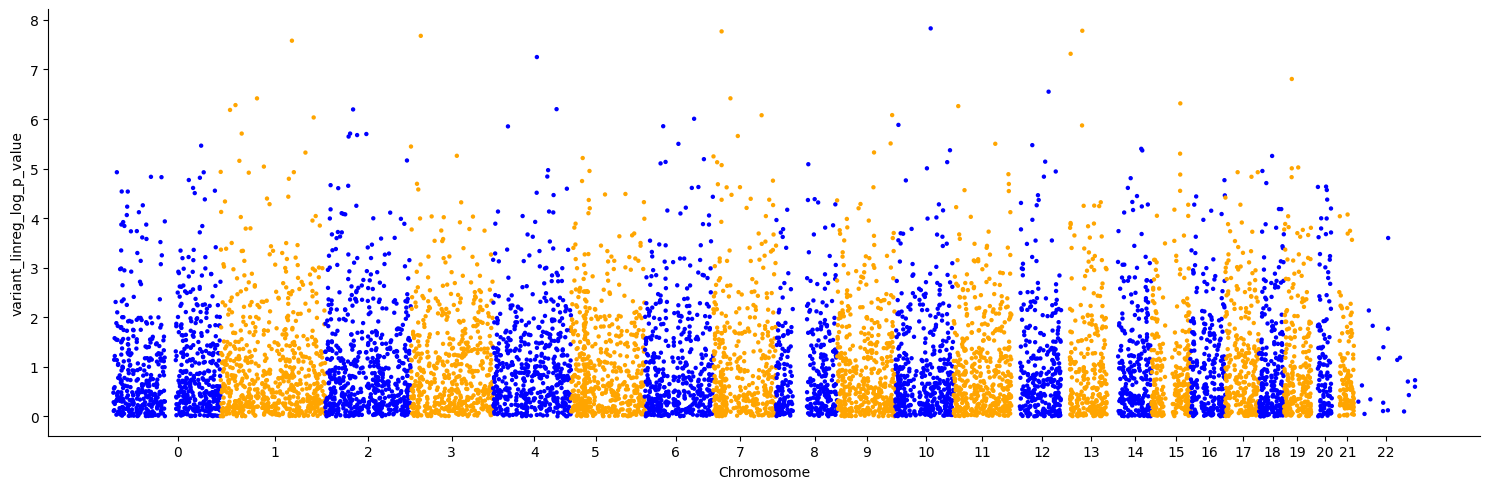
import math
import matplotlib.pyplot as plt

def qq_plot(ds):
    p = ds["variant_linreg_p_value"].squeeze().values
    p.sort()
    n = len(p)
    expected_p = -np.log10(np.arange(1, n + 1) / n)
    observed_p = -np.log10(p)
    max_val = math.ceil(max(np.max(expected_p), np.max(observed_p)))

    df = pd.DataFrame({"Expected -log10(p)": expected_p, "Observed -log10(p)": observed_p})

    fig, ax = plt.subplots(figsize=(12, 12));
    g = sns.scatterplot(data=df, x="Expected -log10(p)", y="Observed -log10(p)", ax=ax, linewidth=0)

    x_pred = np.linspace(0, max_val, 50)
    sns.lineplot(x=x_pred, y=x_pred, ax=ax)

    g.set(xlim=(0, max_val), ylim=(0, max_val))
qq_plot(ds_lr)
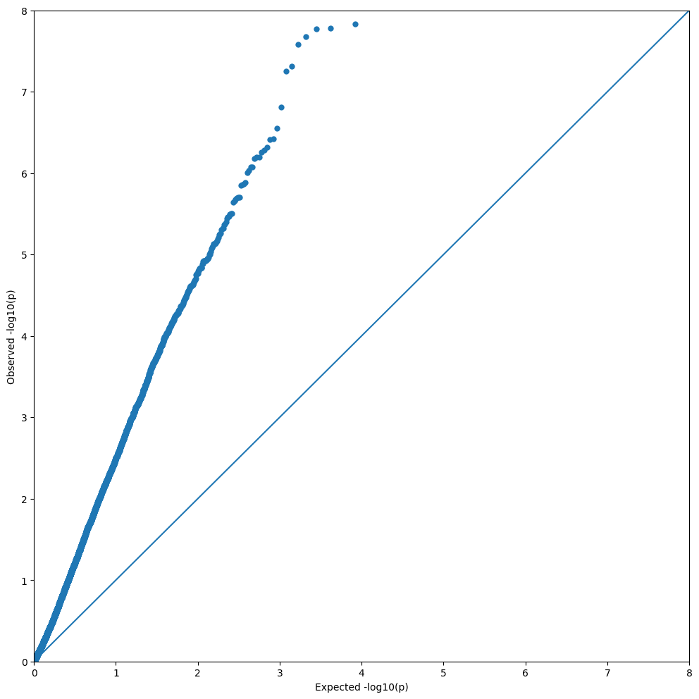
Confounded!#
As explained in the Hail tutorial, the data contains a confounder, so it is necessary to include ancestry as a covariate in the linear regression.
Rather than just use the reported ancestry, it’s better to use principal components from running a PCA on the data.
ds_pca = sg.stats.pca.count_call_alternate_alleles(ds)
# To run PCA we need to filter out variants with any missing alt allele counts
# Or where the counts are zero for all samples
variant_mask = ((ds_pca.call_alternate_allele_count < 0).any(dim="samples")) | \
    (ds_pca.call_alternate_allele_count.std(dim="samples") <= 0.0)
ds_pca = ds_pca.sel(variants=~variant_mask)
ds_pca = sg.pca(ds_pca)
ds_pca.sample_pca_projection.values
array([[ -8.453594 , -26.128803 , -11.008166 , ..., -14.801221 ,
         24.537298 ,  -1.0794897],
       [ -9.496218 , -26.319613 , -10.1165   , ...,   1.6827631,
          7.6817007,  -5.957279 ],
       [ -7.8734055, -25.404316 ,  -9.859188 , ...,   4.382868 ,
         -9.368454 ,   6.384339 ],
       ...,
       [-10.974406 , -11.576627 ,  20.12465  , ...,  -4.4210625,
         -0.5393095,   1.0124536],
       [-10.754403 , -11.41477  ,  15.3587885, ...,   1.795162 ,
          3.4263666,  -7.985671 ],
       [-13.062881 , -11.688105 ,  16.351276 , ...,  -7.2050476,
         -1.7339797,   5.175017 ]], dtype=float32)
ds_pca
<xarray.Dataset>
Dimensions:                              (samples: 250, components: 10,
                                          variants: 3491, genotypes: 3,
                                          alleles: 2, ploidy: 2, contigs: 84,
                                          filters: 1)
Coordinates:
  * genotypes                            (genotypes) <U3 '0/0' '0/1' '1/1'
Dimensions without coordinates: samples, components, variants, alleles, ploidy,
                                contigs, filters
Data variables: (12/48)
    sample_pca_projection                (samples, components) float32 dask.array<chunksize=(250, 10), meta=np.ndarray>
    sample_pca_component                 (variants, components) float32 dask.array<chunksize=(3325, 10), meta=np.ndarray>
    sample_pca_explained_variance        (components) float32 dask.array<chunksize=(10,), meta=np.ndarray>
    sample_pca_explained_variance_ratio  (components) float32 dask.array<chunksize=(10,), meta=np.ndarray>
    sample_pca_loading                   (variants, components) float32 dask.array<chunksize=(3325, 10), meta=np.ndarray>
    call_alternate_allele_count          (variants, samples) int16 dask.array<chunksize=(3325, 250), meta=np.ndarray>
    ...                                   ...
    SuperPopulation                      (samples) object 'EUR' 'EUR' ... 'SAS'
    isFemale                             (samples) bool False True ... True
    PurpleHair                           (samples) bool False False ... True
    CaffeineConsumption                  (samples) int64 4 4 4 3 6 ... 6 4 6 5 5
    sample_dp_mean                       (samples) float64 dask.array<chunksize=(250,), meta=np.ndarray>
    call_dosage                          (variants, samples) int64 dask.array<chunksize=(3325, 250), meta=np.ndarray>
Attributes: (7)- samples: 250
- components: 10
- variants: 3491
- genotypes: 3
- alleles: 2
- ploidy: 2
- contigs: 84
- filters: 1
- genotypes(genotypes)<U3'0/0' '0/1' '1/1'
array(['0/0', '0/1', '1/1'], dtype='<U3')
- sample_pca_projection(samples, components)float32dask.array<chunksize=(250, 10), meta=np.ndarray>
Array Chunk Bytes 9.77 kiB 9.77 kiB Shape (250, 10) (250, 10) Count 65 Graph Layers 1 Chunks Type float32 numpy.ndarray - sample_pca_component(variants, components)float32dask.array<chunksize=(3325, 10), meta=np.ndarray>
Array Chunk Bytes 136.37 kiB 129.88 kiB Shape (3491, 10) (3325, 10) Count 62 Graph Layers 2 Chunks Type float32 numpy.ndarray - sample_pca_explained_variance(components)float32dask.array<chunksize=(10,), meta=np.ndarray>
Array Chunk Bytes 40 B 40 B Shape (10,) (10,) Count 65 Graph Layers 1 Chunks Type float32 numpy.ndarray - sample_pca_explained_variance_ratio(components)float32dask.array<chunksize=(10,), meta=np.ndarray>
Array Chunk Bytes 40 B 40 B Shape (10,) (10,) Count 70 Graph Layers 1 Chunks Type float32 numpy.ndarray - sample_pca_loading(variants, components)float32dask.array<chunksize=(3325, 10), meta=np.ndarray>
Array Chunk Bytes 136.37 kiB 129.88 kiB Shape (3491, 10) (3325, 10) Count 71 Graph Layers 2 Chunks Type float32 numpy.ndarray - call_alternate_allele_count(variants, samples)int16dask.array<chunksize=(3325, 250), meta=np.ndarray>
Array Chunk Bytes 1.66 MiB 1.59 MiB Shape (3491, 250) (3325, 250) Count 18 Graph Layers 2 Chunks Type int16 numpy.ndarray - variant_hwe_p_value(variants)float64dask.array<chunksize=(3325,), meta=np.ndarray>
- comment :
- P values from HWE test for each variant as float in [0, 1].
Array Chunk Bytes 27.27 kiB 25.98 kiB Shape (3491,) (3325,) Count 10 Graph Layers 2 Chunks Type float64 numpy.ndarray - variant_genotype_count(variants, genotypes)uint64dask.array<chunksize=(3325, 3), meta=np.ndarray>
- comment :
- The number of observations for each possible genotype at each variant. Counts are sorted following the ordering defined in the VCF specification. - For biallelic, diploid genotypes the ordering is ``00``, ``01``, ``11`` (homozygous reference, heterozygous, homozygous alternate). - For triallelic, diploid genotypes the ordering is ``00``, ``01``, ``11``, ``02``, ``12``, ``22`` - For triallelic, triploid genotypes the ordering is ``000``, ``001``, ``011``, ``111``, ``002``, ``012``, ``112``, ``022``, ``122``, ``222``
Array Chunk Bytes 81.82 kiB 77.93 kiB Shape (3491, 3) (3325, 3) Count 6 Graph Layers 2 Chunks Type uint64 numpy.ndarray - genotype_id(genotypes)<U3dask.array<chunksize=(3,), meta=np.ndarray>
- comment :
- VCF style genotype strings for all possible genotypes given the size of the ploidy and alleles dimensions. The ordering of genotype strings follows the ordering outlined in the VCF specification for arrays of size "G".
Array Chunk Bytes 36 B 36 B Shape (3,) (3,) Count 4 Graph Layers 1 Chunks Type numpy.ndarray - variant_n_called(variants)int64dask.array<chunksize=(3325,), meta=np.ndarray>
- comment :
- The number of samples with called genotypes.
Array Chunk Bytes 27.27 kiB 25.98 kiB Shape (3491,) (3325,) Count 10 Graph Layers 2 Chunks Type int64 numpy.ndarray - variant_call_rate(variants)float64dask.array<chunksize=(3325,), meta=np.ndarray>
- comment :
- The fraction of samples with called genotypes.
Array Chunk Bytes 27.27 kiB 25.98 kiB Shape (3491,) (3325,) Count 11 Graph Layers 2 Chunks Type float64 numpy.ndarray - variant_n_het(variants)int64dask.array<chunksize=(3325,), meta=np.ndarray>
- comment :
- The number of samples with heterozygous calls.
Array Chunk Bytes 27.27 kiB 25.98 kiB Shape (3491,) (3325,) Count 26 Graph Layers 2 Chunks Type int64 numpy.ndarray - variant_n_hom_ref(variants)int64dask.array<chunksize=(3325,), meta=np.ndarray>
- comment :
- The number of samples with homozygous reference calls.
Array Chunk Bytes 27.27 kiB 25.98 kiB Shape (3491,) (3325,) Count 16 Graph Layers 2 Chunks Type int64 numpy.ndarray - variant_n_hom_alt(variants)int64dask.array<chunksize=(3325,), meta=np.ndarray>
- comment :
- The number of samples with homozygous alternate calls.
Array Chunk Bytes 27.27 kiB 25.98 kiB Shape (3491,) (3325,) Count 21 Graph Layers 2 Chunks Type int64 numpy.ndarray - variant_n_non_ref(variants)int64dask.array<chunksize=(3325,), meta=np.ndarray>
- comment :
- The number of samples that are not homozygous reference calls.
Array Chunk Bytes 27.27 kiB 25.98 kiB Shape (3491,) (3325,) Count 16 Graph Layers 2 Chunks Type int64 numpy.ndarray - variant_allele_count(variants, alleles)uint64dask.array<chunksize=(3325, 2), meta=np.ndarray>
- comment :
- Variant allele counts. With shape (variants, alleles) and values corresponding to the number of non-missing occurrences of each allele.
Array Chunk Bytes 54.55 kiB 51.95 kiB Shape (3491, 2) (3325, 2) Count 8 Graph Layers 2 Chunks Type uint64 numpy.ndarray - variant_allele_total(variants)int64dask.array<chunksize=(3325,), meta=np.ndarray>
- comment :
- The number of occurrences of all alleles.
Array Chunk Bytes 27.27 kiB 25.98 kiB Shape (3491,) (3325,) Count 9 Graph Layers 2 Chunks Type int64 numpy.ndarray - variant_allele_frequency(variants, alleles)float64dask.array<chunksize=(3325, 2), meta=np.ndarray>
- comment :
- The frequency of the occurrence of each allele.
Array Chunk Bytes 54.55 kiB 51.95 kiB Shape (3491, 2) (3325, 2) Count 18 Graph Layers 2 Chunks Type float64 numpy.ndarray - sample_n_called(samples)int64dask.array<chunksize=(250,), meta=np.ndarray>
- comment :
- The number of variants with called genotypes.
Array Chunk Bytes 1.95 kiB 1.95 kiB Shape (250,) (250,) Count 8 Graph Layers 1 Chunks Type int64 numpy.ndarray - sample_call_rate(samples)float64dask.array<chunksize=(250,), meta=np.ndarray>
- comment :
- The fraction of variants with called genotypes.
- long_name :
- Sample call rate
Array Chunk Bytes 1.95 kiB 1.95 kiB Shape (250,) (250,) Count 9 Graph Layers 1 Chunks Type float64 numpy.ndarray - sample_n_het(samples)int64dask.array<chunksize=(250,), meta=np.ndarray>
- comment :
- The number of variants with heterozygous calls.
Array Chunk Bytes 1.95 kiB 1.95 kiB Shape (250,) (250,) Count 23 Graph Layers 1 Chunks Type int64 numpy.ndarray - sample_n_hom_ref(samples)int64dask.array<chunksize=(250,), meta=np.ndarray>
- comment :
- The number of variants with homozygous reference calls.
Array Chunk Bytes 1.95 kiB 1.95 kiB Shape (250,) (250,) Count 13 Graph Layers 1 Chunks Type int64 numpy.ndarray - sample_n_hom_alt(samples)int64dask.array<chunksize=(250,), meta=np.ndarray>
- comment :
- The number of variants with homozygous alternate calls.
Array Chunk Bytes 1.95 kiB 1.95 kiB Shape (250,) (250,) Count 18 Graph Layers 1 Chunks Type int64 numpy.ndarray - sample_n_non_ref(samples)int64dask.array<chunksize=(250,), meta=np.ndarray>
- comment :
- The number of variants that are not homozygous reference calls.
Array Chunk Bytes 1.95 kiB 1.95 kiB Shape (250,) (250,) Count 13 Graph Layers 1 Chunks Type int64 numpy.ndarray - call_AD(variants, samples, alleles)int32dask.array<chunksize=(3325, 250, 2), meta=np.ndarray>
Array Chunk Bytes 6.66 MiB 6.34 MiB Shape (3491, 250, 2) (3325, 250, 2) Count 5 Graph Layers 2 Chunks Type int32 numpy.ndarray - call_DP(variants, samples)int32dask.array<chunksize=(3325, 250), meta=np.ndarray>
Array Chunk Bytes 3.33 MiB 3.17 MiB Shape (3491, 250) (3325, 250) Count 5 Graph Layers 2 Chunks Type int32 numpy.ndarray - call_GQ(variants, samples)int32dask.array<chunksize=(3325, 250), meta=np.ndarray>
Array Chunk Bytes 3.33 MiB 3.17 MiB Shape (3491, 250) (3325, 250) Count 5 Graph Layers 2 Chunks Type int32 numpy.ndarray - call_genotype(variants, samples, ploidy)int8dask.array<chunksize=(3325, 250, 2), meta=np.ndarray>
- comment :
- Call genotype. Encoded as allele values (0 for the reference, 1 for the first allele, 2 for the second allele), -1 to indicate a missing value, or -2 to indicate a non allele in mixed ploidy datasets.
- mixed_ploidy :
- False
Array Chunk Bytes 1.66 MiB 1.59 MiB Shape (3491, 250, 2) (3325, 250, 2) Count 5 Graph Layers 2 Chunks Type int8 numpy.ndarray - call_genotype_mask(variants, samples, ploidy)booldask.array<chunksize=(3325, 250, 2), meta=np.ndarray>
- comment :
- A flag for each call indicating which values are missing.
Array Chunk Bytes 1.66 MiB 1.59 MiB Shape (3491, 250, 2) (3325, 250, 2) Count 5 Graph Layers 2 Chunks Type bool numpy.ndarray - call_genotype_phased(variants, samples)booldask.array<chunksize=(3325, 250), meta=np.ndarray>
- comment :
- A flag for each call indicating if it is phased or not. If omitted all calls are unphased.
Array Chunk Bytes 852.29 kiB 811.77 kiB Shape (3491, 250) (3325, 250) Count 5 Graph Layers 2 Chunks Type bool numpy.ndarray - contig_id(contigs)<U10dask.array<chunksize=(84,), meta=np.ndarray>
- comment :
- Contig identifiers.
Array Chunk Bytes 3.28 kiB 3.28 kiB Shape (84,) (84,) Count 2 Graph Layers 1 Chunks Type numpy.ndarray - contig_length(contigs)int64dask.array<chunksize=(84,), meta=np.ndarray>
Array Chunk Bytes 672 B 672 B Shape (84,) (84,) Count 2 Graph Layers 1 Chunks Type int64 numpy.ndarray - filter_id(filters)objectdask.array<chunksize=(1,), meta=np.ndarray>
Array Chunk Bytes 8 B 8 B Shape (1,) (1,) Count 2 Graph Layers 1 Chunks Type object numpy.ndarray - variant_allele(variants, alleles)objectdask.array<chunksize=(3325, 2), meta=np.ndarray>
- comment :
- The possible alleles for the variant.
Array Chunk Bytes 54.55 kiB 51.95 kiB Shape (3491, 2) (3325, 2) Count 4 Graph Layers 2 Chunks Type object numpy.ndarray - variant_contig(variants)int8dask.array<chunksize=(3325,), meta=np.ndarray>
- comment :
- Index corresponding to contig name for each variant. In some less common scenarios, this may also be equivalent to the contig names if the data generating process used contig names that were also integers.
Array Chunk Bytes 3.41 kiB 3.25 kiB Shape (3491,) (3325,) Count 4 Graph Layers 2 Chunks Type int8 numpy.ndarray - variant_filter(variants, filters)booldask.array<chunksize=(3325, 1), meta=np.ndarray>
Array Chunk Bytes 3.41 kiB 3.25 kiB Shape (3491, 1) (3325, 1) Count 4 Graph Layers 2 Chunks Type bool numpy.ndarray - variant_id(variants)objectdask.array<chunksize=(3325,), meta=np.ndarray>
- comment :
- The unique identifier of the variant.
Array Chunk Bytes 27.27 kiB 25.98 kiB Shape (3491,) (3325,) Count 4 Graph Layers 2 Chunks Type object numpy.ndarray - variant_id_mask(variants)booldask.array<chunksize=(3325,), meta=np.ndarray>
Array Chunk Bytes 3.41 kiB 3.25 kiB Shape (3491,) (3325,) Count 4 Graph Layers 2 Chunks Type bool numpy.ndarray - variant_position(variants)int32dask.array<chunksize=(3325,), meta=np.ndarray>
- comment :
- The reference position of the variant.
Array Chunk Bytes 13.64 kiB 12.99 kiB Shape (3491,) (3325,) Count 4 Graph Layers 2 Chunks Type int32 numpy.ndarray - variant_quality(variants)float32dask.array<chunksize=(3325,), meta=np.ndarray>
Array Chunk Bytes 13.64 kiB 12.99 kiB Shape (3491,) (3325,) Count 4 Graph Layers 2 Chunks Type float32 numpy.ndarray - variant_contig_name(variants)int640 0 0 0 0 0 0 ... 21 21 21 21 21 22
array([ 0, 0, 0, ..., 21, 21, 22])
- Population(samples)object'GBR' 'GBR' 'GBR' ... 'GIH' 'GIH'
array(['GBR', 'GBR', 'GBR', 'GBR', 'GBR', 'GBR', 'GBR', 'FIN', 'FIN', 'FIN', 'CHS', 'CHS', 'CHS', 'CHS', 'CHS', 'CHS', 'CHS', 'CHS', 'CHS', 'CHS', 'CHS', 'CHS', 'PUR', 'CDX', 'PUR', 'PUR', 'PUR', 'PUR', 'PUR', 'PUR', 'PUR', 'CLM', 'CLM', 'CLM', 'GBR', 'CLM', 'PUR', 'CLM', 'CLM', 'CLM', 'IBS', 'PEL', 'IBS', 'IBS', 'IBS', 'IBS', 'IBS', 'GBR', 'CDX', 'CDX', 'CDX', 'CDX', 'CDX', 'CDX', 'KHV', 'KHV', 'KHV', 'KHV', 'KHV', 'ACB', 'PEL', 'PEL', 'PEL', 'PEL', 'ACB', 'KHV', 'ACB', 'KHV', 'KHV', 'KHV', 'KHV', 'KHV', 'CDX', 'CDX', 'CDX', 'IBS', 'IBS', 'CDX', 'PEL', 'PEL', 'PEL', 'CDX', 'CDX', 'CDX', 'CDX', 'CDX', 'CDX', 'CDX', 'CDX', 'CDX', 'ACB', 'GWD', 'GWD', 'ACB', 'KHV', 'GWD', 'GWD', 'ACB', 'GWD', 'PJL', 'GWD', 'PJL', 'PJL', 'PJL', 'PJL', 'PJL', 'GWD', 'GWD', 'GWD', 'PJL', 'GWD', 'GWD', 'GWD', 'GWD', 'GWD', 'GWD', 'ESN', 'ESN', 'BEB', 'GWD', 'MSL', 'MSL', 'ESN', 'ESN', 'ESN', 'MSL', 'PJL', 'GWD', 'GWD', 'GWD', 'ESN', 'ESN', 'ESN', 'ESN', 'MSL', 'MSL', 'MSL', 'MSL', 'PJL', 'PJL', 'ESN', 'MSL', 'MSL', 'BEB', 'BEB', 'BEB', 'PJL', 'STU', 'STU', 'STU', 'ITU', 'STU', 'STU', 'BEB', 'BEB', 'BEB', 'STU', 'ITU', 'STU', 'BEB', 'BEB', 'STU', 'ITU', 'ITU', 'ITU', 'ITU', 'STU', 'BEB', 'BEB', 'ITU', 'STU', 'STU', 'ITU', 'CEU', 'CEU', 'CEU', 'CEU', 'CEU', 'CEU', 'CEU', 'CEU', 'CEU', 'CEU', 'YRI', 'CHB', 'CHB', 'CHB', 'CHB', 'CHB', 'CHB', 'CHB', 'YRI', 'YRI', 'YRI', 'JPT', 'JPT', 'JPT', 'JPT', 'JPT', 'JPT', 'JPT', 'JPT', 'JPT', 'JPT', 'YRI', 'YRI', 'YRI', 'YRI', 'LWK', 'LWK', 'LWK', 'LWK', 'LWK', 'LWK', 'LWK', 'LWK', 'LWK', 'MXL', 'MXL', 'MXL', 'MXL', 'MXL', 'ASW', 'MXL', 'MXL', 'MXL', 'ASW', 'ASW', 'TSI', 'TSI', 'TSI', 'TSI', 'TSI', 'TSI', 'TSI', 'TSI', 'TSI', 'GIH', 'GIH', 'GIH', 'GIH', 'GIH', 'GIH', 'GIH', 'GIH', 'GIH', 'GIH', 'GIH', 'GIH', 'GIH'], dtype=object) - SuperPopulation(samples)object'EUR' 'EUR' 'EUR' ... 'SAS' 'SAS'
array(['EUR', 'EUR', 'EUR', 'EUR', 'EUR', 'EUR', 'EUR', 'EUR', 'EUR', 'EUR', 'EAS', 'EAS', 'EAS', 'EAS', 'EAS', 'EAS', 'EAS', 'EAS', 'EAS', 'EAS', 'EAS', 'EAS', 'AMR', 'EAS', 'AMR', 'AMR', 'AMR', 'AMR', 'AMR', 'AMR', 'AMR', 'AMR', 'AMR', 'AMR', 'EUR', 'AMR', 'AMR', 'AMR', 'AMR', 'AMR', 'EUR', 'AMR', 'EUR', 'EUR', 'EUR', 'EUR', 'EUR', 'EUR', 'EAS', 'EAS', 'EAS', 'EAS', 'EAS', 'EAS', 'EAS', 'EAS', 'EAS', 'EAS', 'EAS', 'AFR', 'AMR', 'AMR', 'AMR', 'AMR', 'AFR', 'EAS', 'AFR', 'EAS', 'EAS', 'EAS', 'EAS', 'EAS', 'EAS', 'EAS', 'EAS', 'EUR', 'EUR', 'EAS', 'AMR', 'AMR', 'AMR', 'EAS', 'EAS', 'EAS', 'EAS', 'EAS', 'EAS', 'EAS', 'EAS', 'EAS', 'AFR', 'AFR', 'AFR', 'AFR', 'EAS', 'AFR', 'AFR', 'AFR', 'AFR', 'SAS', 'AFR', 'SAS', 'SAS', 'SAS', 'SAS', 'SAS', 'AFR', 'AFR', 'AFR', 'SAS', 'AFR', 'AFR', 'AFR', 'AFR', 'AFR', 'AFR', 'AFR', 'AFR', 'SAS', 'AFR', 'AFR', 'AFR', 'AFR', 'AFR', 'AFR', 'AFR', 'SAS', 'AFR', 'AFR', 'AFR', 'AFR', 'AFR', 'AFR', 'AFR', 'AFR', 'AFR', 'AFR', 'AFR', 'SAS', 'SAS', 'AFR', 'AFR', 'AFR', 'SAS', 'SAS', 'SAS', 'SAS', 'SAS', 'SAS', 'SAS', 'SAS', 'SAS', 'SAS', 'SAS', 'SAS', 'SAS', 'SAS', 'SAS', 'SAS', 'SAS', 'SAS', 'SAS', 'SAS', 'SAS', 'SAS', 'SAS', 'SAS', 'SAS', 'SAS', 'SAS', 'SAS', 'SAS', 'SAS', 'EUR', 'EUR', 'EUR', 'EUR', 'EUR', 'EUR', 'EUR', 'EUR', 'EUR', 'EUR', 'AFR', 'EAS', 'EAS', 'EAS', 'EAS', 'EAS', 'EAS', 'EAS', 'AFR', 'AFR', 'AFR', 'EAS', 'EAS', 'EAS', 'EAS', 'EAS', 'EAS', 'EAS', 'EAS', 'EAS', 'EAS', 'AFR', 'AFR', 'AFR', 'AFR', 'AFR', 'AFR', 'AFR', 'AFR', 'AFR', 'AFR', 'AFR', 'AFR', 'AFR', 'AMR', 'AMR', 'AMR', 'AMR', 'AMR', 'AFR', 'AMR', 'AMR', 'AMR', 'AFR', 'AFR', 'EUR', 'EUR', 'EUR', 'EUR', 'EUR', 'EUR', 'EUR', 'EUR', 'EUR', 'SAS', 'SAS', 'SAS', 'SAS', 'SAS', 'SAS', 'SAS', 'SAS', 'SAS', 'SAS', 'SAS', 'SAS', 'SAS'], dtype=object) - isFemale(samples)boolFalse True False ... False True
array([False, True, False, True, False, False, True, False, True, False, False, True, False, True, False, False, False, True, True, True, False, True, True, False, True, True, False, False, True, False, True, False, True, True, False, True, True, False, False, True, True, True, False, True, False, False, True, True, True, True, True, True, True, True, True, False, True, True, True, True, True, True, False, False, True, False, True, True, True, False, False, True, True, True, True, True, False, False, False, True, True, False, False, False, False, False, False, False, False, False, True, True, False, True, False, False, True, True, True, False, True, False, True, True, False, False, True, False, False, False, False, True, True, True, True, False, True, False, False, True, False, True, True, False, False, False, False, True, True, True, True, True, True, False, True, True, False, True, False, True, True, False, True, True, False, True, False, True, False, True, True, False, False, False, False, True, False, True, True, False, True, True, True, True, True, False, True, False, True, True, False, False, False, False, True, False, False, True, False, True, False, False, True, False, True, False, True, True, False, True, False, False, True, True, False, False, True, True, True, False, False, False, False, True, False, False, True, True, True, False, True, False, True, False, True, True, True, False, True, False, True, False, True, False, False, True, False, False, True, False, True, True, True, False, True, False, True, False, False, True, True, True, True, True, False, False, False, False, False, True]) - PurpleHair(samples)boolFalse False False ... True True
array([False, False, False, False, False, True, False, False, True, True, False, False, True, True, True, True, True, True, True, False, True, True, False, False, False, False, False, True, False, True, True, True, False, True, False, True, False, False, False, False, True, False, False, True, False, False, True, True, False, True, False, False, False, False, False, True, True, False, False, True, True, True, False, False, True, False, True, True, True, True, True, True, True, True, False, True, True, True, True, True, False, False, False, True, False, True, True, False, False, False, False, True, False, True, False, True, True, True, True, True, True, True, False, True, False, False, False, True, True, False, False, True, True, True, True, True, False, False, True, True, False, False, False, False, False, True, False, False, False, False, True, False, False, False, False, False, False, False, False, True, False, False, True, True, True, False, True, False, True, True, True, True, True, True, False, False, False, False, False, False, True, True, True, True, False, False, True, False, True, True, False, False, True, False, False, True, True, True, True, True, True, False, True, True, False, False, True, True, True, False, True, False, False, False, True, True, True, False, False, False, False, False, True, False, False, False, True, False, False, True, False, False, False, False, False, True, False, True, True, False, False, False, False, True, False, True, False, True, True, False, False, False, False, True, True, True, True, True, True, False, False, True, False, False, True, True, True, False, True, True]) - CaffeineConsumption(samples)int644 4 4 3 6 2 2 5 ... 5 6 4 6 4 6 5 5
array([4, 4, 4, 3, 6, 2, 2, 5, 5, 4, 6, 5, 7, 5, 7, 1, 5, 5, 4, 4, 5, 5, 5, 6, 4, 4, 6, 3, 3, 5, 4, 4, 5, 5, 4, 6, 5, 4, 4, 5, 6, 3, 7, 5, 5, 6, 3, 2, 5, 5, 4, 6, 5, 6, 4, 6, 7, 6, 7, 3, 5, 6, 5, 6, 4, 5, 4, 4, 5, 8, 3, 4, 4, 7, 5, 2, 6, 7, 6, 5, 3, 4, 5, 5, 5, 5, 6, 4, 5, 7, 2, 3, 3, 2, 6, 4, 2, 6, 5, 3, 4, 7, 6, 7, 6, 3, 4, 2, 2, 5, 6, 7, 8, 6, 2, 3, 2, 0, 5, 7, 5, 1, 4, 3, 2, 4, 6, 5, 4, 4, 1, 5, 5, 3, 1, 1, 3, 2, 4, 2, 1, 3, 3, 4, 4, 5, 6, 5, 4, 5, 0, 4, 5, 4, 3, 3, 4, 4, 3, 5, 6, 5, 3, 4, 4, 6, 3, 5, 5, 4, 5, 3, 5, 4, 6, 5, 7, 5, 6, 6, 4, 4, 5, 3, 5, 4, 3, 8, 4, 6, 8, 3, 4, 2, 5, 6, 6, 4, 3, 5, 7, 4, 5, 5, 6, 3, 2, 4, 5, 6, 7, 2, 4, 2, 1, 5, 3, 4, 9, 6, 4, 3, 4, 4, 6, 7, 6, 3, 4, 3, 6, 6, 3, 4, 4, 4, 6, 7, 4, 5, 4, 5, 5, 6, 4, 6, 4, 6, 5, 5]) - sample_dp_mean(samples)float64dask.array<chunksize=(250,), meta=np.ndarray>
- long_name :
- Mean Sample DP
Array Chunk Bytes 1.95 kiB 1.95 kiB Shape (250,) (250,) Count 8 Graph Layers 1 Chunks Type float64 numpy.ndarray - call_dosage(variants, samples)int64dask.array<chunksize=(3325, 250), meta=np.ndarray>
Array Chunk Bytes 6.66 MiB 6.34 MiB Shape (3491, 250) (3325, 250) Count 7 Graph Layers 2 Chunks Type int64 numpy.ndarray
- contig_lengths :
- [249250621, 243199373, 198022430, 191154276, 180915260, 171115067, 159138663, 146364022, 141213431, 135534747, 135006516, 133851895, 115169878, 107349540, 102531392, 90354753, 81195210, 78077248, 59128983, 63025520, 48129895, 51304566, 155270560, 59373566, 16569, 4262, 15008, 19913, 27386, 27682, 33824, 34474, 36148, 36422, 36651, 37175, 37498, 38154, 38502, 38914, 39786, 39929, 39939, 40103, 40531, 40652, 41001, 41933, 41934, 42152, 43341, 43523, 43691, 45867, 45941, 81310, 90085, 92689, 106433, 128374, 129120, 137718, 155397, 159169, 161147, 161802, 164239, 166566, 169874, 172149, 172294, 172545, 174588, 179198, 179693, 180455, 182896, 186858, 186861, 187035, 189789, 191469, 211173, 547496]
- contigs :
- ['1', '2', '3', '4', '5', '6', '7', '8', '9', '10', '11', '12', '13', '14', '15', '16', '17', '18', '19', '20', '21', '22', 'X', 'Y', 'MT', 'GL000207.1', 'GL000226.1', 'GL000229.1', 'GL000231.1', 'GL000210.1', 'GL000239.1', 'GL000235.1', 'GL000201.1', 'GL000247.1', 'GL000245.1', 'GL000197.1', 'GL000203.1', 'GL000246.1', 'GL000249.1', 'GL000196.1', 'GL000248.1', 'GL000244.1', 'GL000238.1', 'GL000202.1', 'GL000234.1', 'GL000232.1', 'GL000206.1', 'GL000240.1', 'GL000236.1', 'GL000241.1', 'GL000243.1', 'GL000242.1', 'GL000230.1', 'GL000237.1', 'GL000233.1', 'GL000204.1', 'GL000198.1', 'GL000208.1', 'GL000191.1', 'GL000227.1', 'GL000228.1', 'GL000214.1', 'GL000221.1', 'GL000209.1', 'GL000218.1', 'GL000220.1', 'GL000213.1', 'GL000211.1', 'GL000199.1', 'GL000217.1', 'GL000216.1', 'GL000215.1', 'GL000205.1', 'GL000219.1', 'GL000224.1', 'GL000223.1', 'GL000195.1', 'GL000212.1', 'GL000222.1', 'GL000200.1', 'GL000193.1', 'GL000194.1', 'GL000225.1', 'GL000192.1']
- filters :
- ['PASS']
- max_alt_alleles_seen :
- 1
- source :
- sgkit-0.6.1.dev2+gcc728043
- vcf_header :
- ##fileformat=VCFv4.2 ##FILTER=<ID=PASS,Description="All filters passed"> ##hailversion=0.2-29fbaeaf265e ##FORMAT=<ID=GT,Number=1,Type=String,Description=""> ##FORMAT=<ID=AD,Number=.,Type=Integer,Description=""> ##FORMAT=<ID=DP,Number=1,Type=Integer,Description=""> ##FORMAT=<ID=GQ,Number=1,Type=Integer,Description=""> ##FORMAT=<ID=PL,Number=.,Type=Integer,Description=""> ##INFO=<ID=AC,Number=.,Type=Integer,Description=""> ##INFO=<ID=AF,Number=.,Type=Float,Description=""> ##INFO=<ID=AN,Number=1,Type=Integer,Description=""> ##INFO=<ID=BaseQRankSum,Number=1,Type=Float,Description=""> ##INFO=<ID=ClippingRankSum,Number=1,Type=Float,Description=""> ##INFO=<ID=DP,Number=1,Type=Integer,Description=""> ##INFO=<ID=DS,Number=0,Type=Flag,Description=""> ##INFO=<ID=FS,Number=1,Type=Float,Description=""> ##INFO=<ID=HaplotypeScore,Number=1,Type=Float,Description=""> ##INFO=<ID=InbreedingCoeff,Number=1,Type=Float,Description=""> ##INFO=<ID=MLEAC,Number=.,Type=Integer,Description=""> ##INFO=<ID=MLEAF,Number=.,Type=Float,Description=""> ##INFO=<ID=MQ,Number=1,Type=Float,Description=""> ##INFO=<ID=MQ0,Number=1,Type=Integer,Description=""> ##INFO=<ID=MQRankSum,Number=1,Type=Float,Description=""> ##INFO=<ID=QD,Number=1,Type=Float,Description=""> ##INFO=<ID=ReadPosRankSum,Number=1,Type=Float,Description=""> ##INFO=<ID=set,Number=1,Type=String,Description=""> ##contig=<ID=1,length=249250621,assembly=GRCh37> ##contig=<ID=2,length=243199373,assembly=GRCh37> ##contig=<ID=3,length=198022430,assembly=GRCh37> ##contig=<ID=4,length=191154276,assembly=GRCh37> ##contig=<ID=5,length=180915260,assembly=GRCh37> ##contig=<ID=6,length=171115067,assembly=GRCh37> ##contig=<ID=7,length=159138663,assembly=GRCh37> ##contig=<ID=8,length=146364022,assembly=GRCh37> ##contig=<ID=9,length=141213431,assembly=GRCh37> ##contig=<ID=10,length=135534747,assembly=GRCh37> ##contig=<ID=11,length=135006516,assembly=GRCh37> ##contig=<ID=12,length=133851895,assembly=GRCh37> ##contig=<ID=13,length=115169878,assembly=GRCh37> ##contig=<ID=14,length=107349540,assembly=GRCh37> ##contig=<ID=15,length=102531392,assembly=GRCh37> ##contig=<ID=16,length=90354753,assembly=GRCh37> ##contig=<ID=17,length=81195210,assembly=GRCh37> ##contig=<ID=18,length=78077248,assembly=GRCh37> ##contig=<ID=19,length=59128983,assembly=GRCh37> ##contig=<ID=20,length=63025520,assembly=GRCh37> ##contig=<ID=21,length=48129895,assembly=GRCh37> ##contig=<ID=22,length=51304566,assembly=GRCh37> ##contig=<ID=X,length=155270560,assembly=GRCh37> ##contig=<ID=Y,length=59373566,assembly=GRCh37> ##contig=<ID=MT,length=16569,assembly=GRCh37> ##contig=<ID=GL000207.1,length=4262,assembly=GRCh37> ##contig=<ID=GL000226.1,length=15008,assembly=GRCh37> ##contig=<ID=GL000229.1,length=19913,assembly=GRCh37> ##contig=<ID=GL000231.1,length=27386,assembly=GRCh37> ##contig=<ID=GL000210.1,length=27682,assembly=GRCh37> ##contig=<ID=GL000239.1,length=33824,assembly=GRCh37> ##contig=<ID=GL000235.1,length=34474,assembly=GRCh37> ##contig=<ID=GL000201.1,length=36148,assembly=GRCh37> ##contig=<ID=GL000247.1,length=36422,assembly=GRCh37> ##contig=<ID=GL000245.1,length=36651,assembly=GRCh37> ##contig=<ID=GL000197.1,length=37175,assembly=GRCh37> ##contig=<ID=GL000203.1,length=37498,assembly=GRCh37> ##contig=<ID=GL000246.1,length=38154,assembly=GRCh37> ##contig=<ID=GL000249.1,length=38502,assembly=GRCh37> ##contig=<ID=GL000196.1,length=38914,assembly=GRCh37> ##contig=<ID=GL000248.1,length=39786,assembly=GRCh37> ##contig=<ID=GL000244.1,length=39929,assembly=GRCh37> ##contig=<ID=GL000238.1,length=39939,assembly=GRCh37> ##contig=<ID=GL000202.1,length=40103,assembly=GRCh37> ##contig=<ID=GL000234.1,length=40531,assembly=GRCh37> ##contig=<ID=GL000232.1,length=40652,assembly=GRCh37> ##contig=<ID=GL000206.1,length=41001,assembly=GRCh37> ##contig=<ID=GL000240.1,length=41933,assembly=GRCh37> ##contig=<ID=GL000236.1,length=41934,assembly=GRCh37> ##contig=<ID=GL000241.1,length=42152,assembly=GRCh37> ##contig=<ID=GL000243.1,length=43341,assembly=GRCh37> ##contig=<ID=GL000242.1,length=43523,assembly=GRCh37> ##contig=<ID=GL000230.1,length=43691,assembly=GRCh37> ##contig=<ID=GL000237.1,length=45867,assembly=GRCh37> ##contig=<ID=GL000233.1,length=45941,assembly=GRCh37> ##contig=<ID=GL000204.1,length=81310,assembly=GRCh37> ##contig=<ID=GL000198.1,length=90085,assembly=GRCh37> ##contig=<ID=GL000208.1,length=92689,assembly=GRCh37> ##contig=<ID=GL000191.1,length=106433,assembly=GRCh37> ##contig=<ID=GL000227.1,length=128374,assembly=GRCh37> ##contig=<ID=GL000228.1,length=129120,assembly=GRCh37> ##contig=<ID=GL000214.1,length=137718,assembly=GRCh37> ##contig=<ID=GL000221.1,length=155397,assembly=GRCh37> ##contig=<ID=GL000209.1,length=159169,assembly=GRCh37> ##contig=<ID=GL000218.1,length=161147,assembly=GRCh37> ##contig=<ID=GL000220.1,length=161802,assembly=GRCh37> ##contig=<ID=GL000213.1,length=164239,assembly=GRCh37> ##contig=<ID=GL000211.1,length=166566,assembly=GRCh37> ##contig=<ID=GL000199.1,length=169874,assembly=GRCh37> ##contig=<ID=GL000217.1,length=172149,assembly=GRCh37> ##contig=<ID=GL000216.1,length=172294,assembly=GRCh37> ##contig=<ID=GL000215.1,length=172545,assembly=GRCh37> ##contig=<ID=GL000205.1,length=174588,assembly=GRCh37> ##contig=<ID=GL000219.1,length=179198,assembly=GRCh37> ##contig=<ID=GL000224.1,length=179693,assembly=GRCh37> ##contig=<ID=GL000223.1,length=180455,assembly=GRCh37> ##contig=<ID=GL000195.1,length=182896,assembly=GRCh37> ##contig=<ID=GL000212.1,length=186858,assembly=GRCh37> ##contig=<ID=GL000222.1,length=186861,assembly=GRCh37> ##contig=<ID=GL000200.1,length=187035,assembly=GRCh37> ##contig=<ID=GL000193.1,length=189789,assembly=GRCh37> ##contig=<ID=GL000194.1,length=191469,assembly=GRCh37> ##contig=<ID=GL000225.1,length=211173,assembly=GRCh37> ##contig=<ID=GL000192.1,length=547496,assembly=GRCh37> #CHROM POS ID REF ALT QUAL FILTER INFO FORMAT HG00096 HG00099 HG00105 HG00118 HG00129 HG00148 HG00177 HG00182 HG00242 HG00254 HG00265 HG00271 HG00274 HG00332 HG00335 HG00369 HG00421 HG00436 HG00452 HG00472 HG00530 HG00534 HG00583 HG00590 HG00598 HG00607 HG00619 HG00623 HG00657 HG00663 HG00704 HG00705 HG00733 HG00864 HG00881 HG01052 HG01070 HG01075 HG01164 HG01174 HG01241 HG01248 HG01256 HG01275 HG01284 HG01334 HG01348 HG01396 HG01443 HG01491 HG01498 HG01537 HG01572 HG01606 HG01623 HG01630 HG01783 HG01784 HG01790 HG01799 HG01801 HG01806 HG01812 HG01813 HG01817 HG01848 HG01849 HG01857 HG01863 HG01874 HG01915 HG01924 HG01965 HG01970 HG01991 HG02010 HG02020 HG02054 HG02086 HG02087 HG02116 HG02122 HG02130 HG02131 HG02152 HG02154 HG02165 HG02224 HG02232 HG02236 HG02250 HG02259 HG02298 HG02318 HG02345 HG02351 HG02363 HG02373 HG02383 HG02384 HG02386 HG02388 HG02389 HG02397 HG02419 HG02462 HG02464 HG02497 HG02511 HG02521 HG02561 HG02574 HG02580 HG02595 HG02603 HG02629 HG02651 HG02682 HG02688 HG02690 HG02699 HG02760 HG02768 HG02771 HG02792 HG02798 HG02811 HG02814 HG02840 HG02870 HG02881 HG02970 HG02973 HG03009 HG03046 HG03074 HG03091 HG03105 HG03127 HG03193 HG03224 HG03237 HG03241 HG03247 HG03259 HG03267 HG03354 HG03366 HG03367 HG03380 HG03419 HG03449 HG03451 HG03458 HG03490 HG03491 HG03511 HG03556 HG03563 HG03598 HG03603 HG03607 HG03636 HG03684 HG03686 HG03690 HG03731 HG03740 HG03755 HG03800 HG03815 HG03832 HG03850 HG03873 HG03897 HG03905 HG03937 HG03948 HG03973 HG04054 HG04059 HG04063 HG04096 HG04099 HG04140 HG04171 HG04209 HG04210 HG04229 HG04239 NA07347 NA11918 NA11919 NA12045 NA12273 NA12342 NA12414 NA12546 NA12760 NA12878 NA18516 NA18525 NA18534 NA18541 NA18557 NA18565 NA18616 NA18619 NA18623 NA18630 NA18631 NA18740 NA18853 NA18865 NA18873 NA18874 NA18916 NA18960 NA18966 NA18975 NA18976 NA18978 NA18990 NA19060 NA19063 NA19076 NA19086 NA19087 NA19096 NA19113 NA19118 NA19185 NA19209 NA19311 NA19314 NA19317 NA19321 NA19379 NA19384 NA19390 NA19397 NA19399 NA19404 NA19446 NA19448 NA19455 NA19456 NA19466 NA19655 NA19657 NA19670 NA19678 NA19679 NA19701 NA19720 NA19756 NA19761 NA19764 NA19786 NA20318 NA20351 NA20517 NA20518 NA20529 NA20587 NA20757 NA20798 NA20799 NA20800 NA20810 NA20826 NA20858 NA20864 NA20869 NA20877 NA20888 NA20910 NA21101 NA21113 NA21114 NA21116 NA21118 NA21133 NA21143
- vcf_zarr_version :
- 0.2
Let’s plot the first two components. Notice how they cluster by ancestry.
ds_pca["sample_pca_projection_0"] = ds_pca.sample_pca_projection[:,0]
ds_pca["sample_pca_projection_1"] = ds_pca.sample_pca_projection[:,1]
ds_pca["sample_pca_projection_2"] = ds_pca.sample_pca_projection[:,2]
ds_pca.plot.scatter(x="sample_pca_projection_0", y="sample_pca_projection_1", hue="SuperPopulation", size=8, s=10);
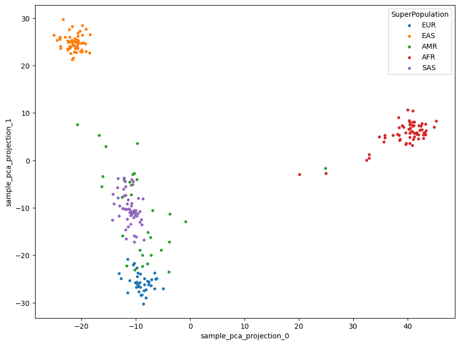
Now we can rerun our linear regression, controlling for sample sex and the first few principal components.
# copy pca components back to dataset with full set of variants to run linear regression again
ds["sample_pca_projection_0"] = ds_pca.sample_pca_projection[:,0]
ds["sample_pca_projection_1"] = ds_pca.sample_pca_projection[:,1]
ds["sample_pca_projection_2"] = ds_pca.sample_pca_projection[:,2]
ds_lr = sg.gwas_linear_regression(ds, dosage="call_dosage",
                                  add_intercept=True,
                                  covariates=["isFemale", "sample_pca_projection_0", "sample_pca_projection_1", "sample_pca_projection_2"],
                                  traits=["CaffeineConsumption"])
qq_plot(ds_lr)
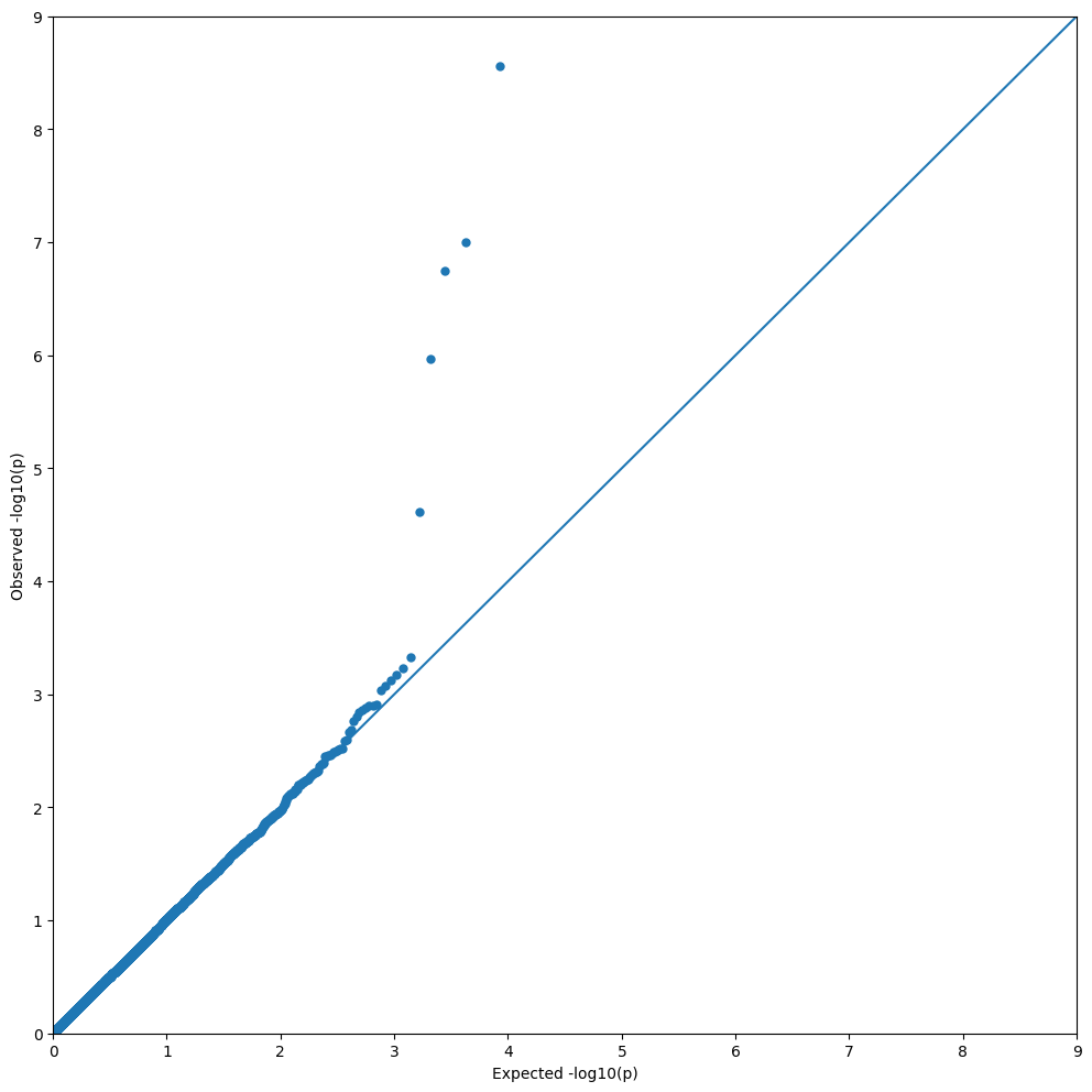
manhattan_plot(ds_lr)
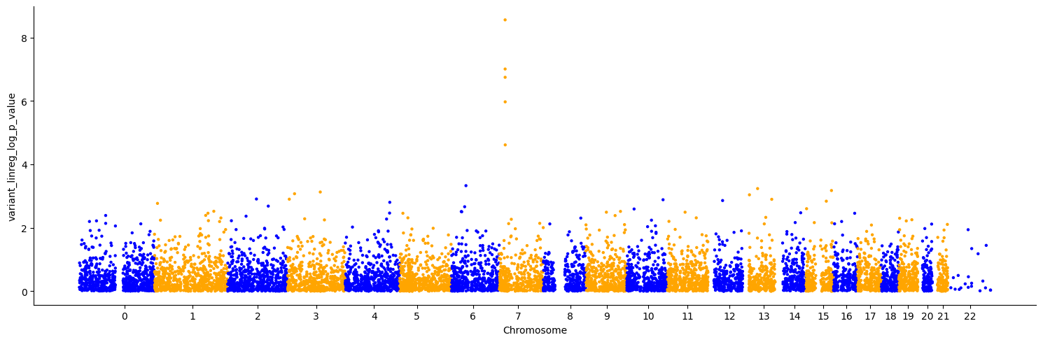
The “caffeine consumption” locus in chromosome 8 is clearly apparent, just like in the Hail tutorial.